Using Empirical Bayes to approximate posteriors for large "black box" estimators
by OMKAR MURALIDHARAN
Many machine learning applications have some kind of regression at their core, so understanding large-scale regression systems is important. But doing this can be hard, for reasons not typically encountered in problems with smaller or less critical regression systems. In this post, we describe the challenges posed by one problem — how to get approximate posteriors — and an approach that we have found useful.
Suppose we want to estimate the number of times an ad will be clicked, or whether a user is looking for images, or the time a user will spend watching a video. All these problems can be phrased as large-scale regressions. We have a collection of items with covariates (i.e. predictive features) and responses (i.e. observed labels), and for each item, we want to estimate a parameter that governs the response. This problem is usually solved by training a big regression system, like a penalized GLM, neural net, or random forest.
Suppose we have $I$ items, each with response $y_i$ and covariates $x_i$ and unknown parameter $\theta_i$, and the responses come from a known parametric family $f_\theta$. We want to estimate the $\theta$s. A black box regression gives us a point estimate of $\theta_i$ for each item, $t_i = t(x_i)$, that is a function of the covariates. However, we often want a posterior for $\theta_i$, not just a point estimate.
Posteriors are useful to understand the system, measure accuracy, and make better decisions. But most common machine learning methods don’t give posteriors, and many don’t have explicit probability models. Methods like the Poisson bootstrap can help us measure the variability of $t$, but don’t give us posteriors either, particularly since good high-dimensional estimators aren’t unbiased.
Exact posteriors are hard to get, but we can get approximate ones by extending calibration, a standard way to post-process regression predictions. There are a few different methods for calibration, but all are based on the same idea: instead of using $t$, estimate and use $E(\theta | t)$. Calibration fixes aggregate bias, which lets us use methods that are efficient but biased. Calibration also scales easily and doesn’t depend on the details of the system producing $t$. That means it can handle the large, changing systems we have to deal with.
The proposed method, which we call second order calibration, goes further and estimates the distribution of $\theta$ around that curve. We don’t observe the true $\theta$s, so we can’t estimate the distribution of $\theta | t$ directly. Instead, we use an Empirical Bayes approach — take the observed $y | t$ distribution and “deconvolve” using the known family $f_\theta$ to infer the distribution of $\theta | t$.
We estimate $G_t$ by standard Empirical Bayes methods, and use it to find interesting posterior quantities such as $\mathrm{var}(\theta | t)$, $E(\theta | t, y)$ and $\mathrm{var}(\theta | t, y)$.
\[
\theta \sim G \\
y | \theta \sim \mathrm{Pois}(N \theta)
\]
Empirical Bayes methods try to estimate $G$ using a collection of responses from a model like the one above. Figure 2 illustrates the idea. The histogram of empirical CTRs ($y_i / N_i$) is spread out with a spike at 0. But much of that dispersion and spikiness is Poisson noise, so the true CTR distribution may look different. Empirical Bayes methods find a prior such that when we add Poisson noise, we fit the distribution of our observed data. In Figure 2, the red line shows a Gamma prior that leads to a good fit. For an introduction to Empirical Bayes, see the paper [3] by Brad Efron (with more in his book [4]).
How exactly should we model $G$? It turns out that if we are interested in the first few posterior moments $\theta | t$ and $\theta | t, y$, the details of the $G$ model don’t really matter. If $G$ fits the marginal distribution of $y$ well and has reasonable tail behavior, our moment estimates will be reasonable (Section 4 of [1] has more details on this). We modeled $G$ using a Gamma distribution. In our application, this simple model was quick to fit using maximum likelihood, and worked as well as a more flexible approach based on mixtures of Gamma distributions (gridded for stability).
We also need to make sure our model fits the data. A simple, necessary check is that the estimated priors lead to marginal distributions that fit the data. This isn’t sufficient, since it doesn’t check our assumed model for the response, $f_\theta$. For example, we might be wrong to assume clicks are Poisson, but a Poisson model could still fit our data with enough freedom in the prior.
One way to check $f_\theta$ is to gather test data and check whether the model fits the relationship between training and test data. This tests the model’s ability to distinguish what is common for each item between the two data sets (the underlying $\theta$) and what is different (the draw from $f_\theta$).
Figure 4 shows the results of such a test. We used our model and training data to construct predictive distributions for test data, and checked where the test data fell in those distributions. If our model were perfect, the test quantiles would be uniform (we jittered the quantiles to account for the discreteness of the data). Our actual quantiles were close to, but not exactly, uniform, indicating a good but not perfect fit.
$E(\theta | t, y)$ balances memorization and generalization to get an improved estimate of $\theta$. For example, suppose we have a query-ad pair with a single impression ($N = 1$). The empirical CTR for that item will be either 0 or 1, and will tell us almost nothing about the true CTR of that ad. In that case, the best we can do is rely on global information and use $E(\theta | t)$ as our estimate. Conversely, suppose we have a query-ad pair with millions of impressions. The empirical CTR tells us much more about the ad’s true CTR than t does, so we should memorize and use $y/N$ as our estimate. The posterior mean smoothly balances memorization and generalization, depending on the amount of information from each source. Doing this in our calibration instead of just relying on $t$ can be more accurate, and can lead to system simplifications. For example, we could use a relatively coarse generalization model for $t$ and rely on calibration to memorize item-specific information.
$\mathrm{var}(\theta | t, y)$ estimates the accuracy of $E(\theta | t, y)$ — this tells us how much we know about each item. These estimates can be useful to make risk-adjusted decisions and explore-exploit trade-offs, or to find situations where the underlying regression method is particularly good or bad.
Second order calibration, like ordinary calibration, is intended to be easy and useful, not comprehensive or optimal, and it shares some of ordinary calibration’s limitations. Both methods can be wrong for slices of the data while being correct on average, since they only use the covariate information through $t$.
Second order calibration also has important additional limitations. We need to know $f_\theta$ to work backwards from the distribution of $y | t$ to that of $\theta | t$. It’s hard to test this assumption directly — a useful indirect check is to make sure the predictive distributions are accurate.
More subtly, second order calibration relies on repeated measurement, in a way that ordinary calibration does not. We must define a unit of observation, and this can be surprisingly tricky. In our CTR example, we defined the unit of observation to be the query-ad pair. But CTR depends on other factors, like the user, and the UI the ad is shown in, and the time of day. It is impossible to refine our unit of observation by all these potential factors and still have repeated measurements for any individual unit. Ordinary calibration and the underlying regression system do not have to solve this problem, since they can just give predictions at the finest-grained level.
We don’t have a fully satisfying answer for this issue. In practice, we have gotten good results by normalizing responses for the first-order effects of factors ignored by our unit definition. More principled solutions could be to account for dispersion within a unit, or to fit some kind of multi-way random effects model.
Second order calibration is a nice example of how dealing with large, complex, changing regression systems requires a different approach. Instead of trying to come up with a principled, correct answer for a particular system, we tried to find something approximate that would work reasonably well without knowing much about the underlying system. The resulting method has clear limitations, but is scalable, maintainable, and accurate enough to be useful.
[1] Omkar Muralidharan, Amir Najmi "Second Order Calibration: A Simple Way To Get Approximate Posteriors", Technical Report, Google, 2015.
[2] H. Brendan McMahan et al, "Ad Click Prediction: a View from the Trenches", Proceedings of the 19th ACM SIGKDD International Conference on Knowledge Discovery and Data Mining (KDD), 2013.
[3] Bradley Efron, "Robbins, Empirical Bayes, and Microarrays", Technical Report, 2003.
[4] Bradley Efron, "Large-Scale Inference: Empirical Bayes Methods for Estimation, Testing, and Prediction", Cambridge University Press, 2013.
Many machine learning applications have some kind of regression at their core, so understanding large-scale regression systems is important. But doing this can be hard, for reasons not typically encountered in problems with smaller or less critical regression systems. In this post, we describe the challenges posed by one problem — how to get approximate posteriors — and an approach that we have found useful.
Suppose we want to estimate the number of times an ad will be clicked, or whether a user is looking for images, or the time a user will spend watching a video. All these problems can be phrased as large-scale regressions. We have a collection of items with covariates (i.e. predictive features) and responses (i.e. observed labels), and for each item, we want to estimate a parameter that governs the response. This problem is usually solved by training a big regression system, like a penalized GLM, neural net, or random forest.
We often use large regressions to make automated decisions. In the examples above, we might use our estimates to choose ads, decide whether to show a user images, or figure out which videos to recommend. These decisions are often business-critical, so it is essential for data scientists to understand and improve the regressions that inform them.
The size and importance of these systems makes this hard. First, systems can be theoretically intractable. Even systems based on well-understood methods usually have custom tweaks to scale or fit the problem better. Second, important systems evolve quickly, since people are constantly trying to improve them. That means any understanding of the system can become out of date.
Thus, the data scientist’s job is to work with a huge black box that can change at any time. This seems impossible. We’ve had some success, however, by ignoring systems’ internal structure and analyzing their predictions. Below, we discuss a way to get approximate posteriors that is based on this approach.
Wanted: approximate posteriors
Suppose we have $I$ items, each with response $y_i$ and covariates $x_i$ and unknown parameter $\theta_i$, and the responses come from a known parametric family $f_\theta$. We want to estimate the $\theta$s. A black box regression gives us a point estimate of $\theta_i$ for each item, $t_i = t(x_i)$, that is a function of the covariates. However, we often want a posterior for $\theta_i$, not just a point estimate.
Exact posteriors are hard to get, but we can get approximate ones by extending calibration, a standard way to post-process regression predictions. There are a few different methods for calibration, but all are based on the same idea: instead of using $t$, estimate and use $E(\theta | t)$. Calibration fixes aggregate bias, which lets us use methods that are efficient but biased. Calibration also scales easily and doesn’t depend on the details of the system producing $t$. That means it can handle the large, changing systems we have to deal with.
Calibration estimates $E(\theta | t)$. We propose estimating the distribution of $\theta | t$ and using this to approximate the distribution of $\theta | x$. Figure 1 illustrates the idea by plotting $\theta$ vs. $t$. Calibration adjusts our estimate, as a function of $t$, by moving from the $y = t$ line to the conditional mean curve $E(\theta | t)$.
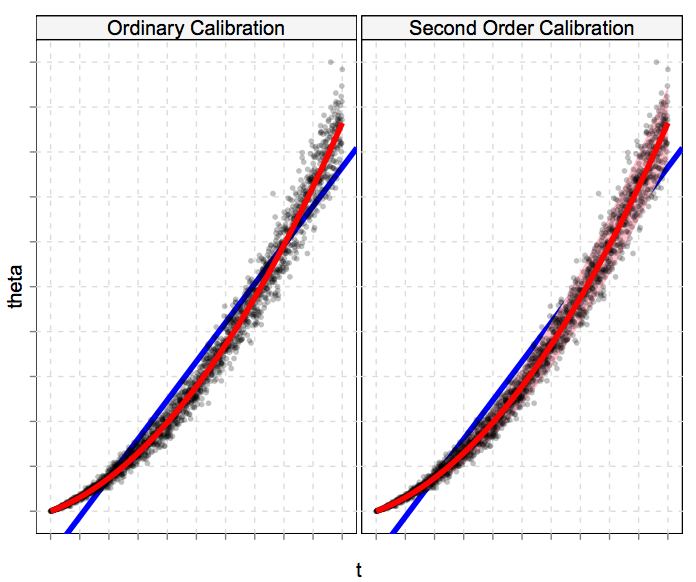 |
| Fig 1: Ordinary and second order calibration. Each panel plots $\theta$ on the y-axis against $t$ on the x-axis. Ordinary calibration, left, adjusts our estimate away from $t$ (the blue line, $y = t$) to $E(\theta|t)$ (the red line). Second order calibration, right, uses $y$ to estimate the distribution of $\theta | t$ (represented by the pink color strip). |
The proposed method, which we call second order calibration, goes further and estimates the distribution of $\theta$ around that curve. We don’t observe the true $\theta$s, so we can’t estimate the distribution of $\theta | t$ directly. Instead, we use an Empirical Bayes approach — take the observed $y | t$ distribution and “deconvolve” using the known family $f_\theta$ to infer the distribution of $\theta | t$.
More precisely, our model is that $\theta$ is drawn from a prior that depends on $t$, then $y$ comes from some known parametric family $f_\theta$. In our model, $\theta$ doesn’t depend directly on $x$ — all the information in $x$ is captured in $t$.
\[
\theta | t \sim G_t \\
y | \theta, t \sim f_\theta
\]
\[
\theta | t \sim G_t \\
y | \theta, t \sim f_\theta
\]
We estimate $G_t$ by standard Empirical Bayes methods, and use it to find interesting posterior quantities such as $\mathrm{var}(\theta | t)$, $E(\theta | t, y)$ and $\mathrm{var}(\theta | t, y)$.
Empirical Bayes posteriors in four easy steps
We’ll explain our method in more detail by applying it to ad click-through-rate (CTR) estimation. Here, our items are query-ad pairs. For example, one item might be a particular ad on the query [flowers]. We observe how often each pair occurs (impressions $N_i$) and is clicked (clicks $y_i$). Our model is that each pair has a true CTR $\theta_i$, and that given impressions and CTR, clicks are Poisson: $y_i|\theta_i \sim \mathrm{Pois}(N_i \theta_i)$ (we can potentially get more clicks than impressions). A machine learning system produces an estimated CTR $t_i$ for each query-ad pair. We discuss this example in detail in our paper [1] on which this post is based. For more on ad CTR estimation, refer to [2].
Our method has four steps:
We could also bin by additional low-dimensional variables that are particularly important. For example, we might bin by $t$ and country. More interestingly, we can bin by $t$ and some estimate of $t$’s variability. This is something we can get from many machine learning systems, either using an internal estimate like a Hessian, or a black box estimate as provided by the Poisson bootstrap.
Our method has four steps:
- Bin by $t$.
- Estimate the prior distribution of $\theta | t$ in each bin using parametric Empirical Bayes.
- Smooth across bins and check fits.
- Calculate posterior quantities of interest.
Step 1: Binning
We eventually want to estimate the $\theta | t$ distributions for each $t$. Since $t$ is continuous, the most natural way would be to use a continuous model. However, we’ve found it easier, and no less effective, to simply bin our query-ad pairs by $t$, so that $t$ is approximately constant in each bin. This means the subsequent fitting steps in each bin can ignore $t$ and can be done in parallel. The computational savings from this approach make the problem much more tractable — we can tackle tens of billions of query-ad pairs in a few hours with a modest number of machines.We could also bin by additional low-dimensional variables that are particularly important. For example, we might bin by $t$ and country. More interestingly, we can bin by $t$ and some estimate of $t$’s variability. This is something we can get from many machine learning systems, either using an internal estimate like a Hessian, or a black box estimate as provided by the Poisson bootstrap.
Step 2: Estimation
We now work within a bin and assume t is effectively constant. Our model thus reduces to\[
\theta \sim G \\
y | \theta \sim \mathrm{Pois}(N \theta)
\]
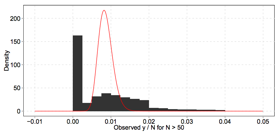 |
| Fig 2: An example of a histogram of $y/N$ and its fitted Gamma prior $G$ (red). The histogram and prior are not supposed to agree: the histogram is the red distribution, plus Poisson noise. |
Empirical Bayes methods try to estimate $G$ using a collection of responses from a model like the one above. Figure 2 illustrates the idea. The histogram of empirical CTRs ($y_i / N_i$) is spread out with a spike at 0. But much of that dispersion and spikiness is Poisson noise, so the true CTR distribution may look different. Empirical Bayes methods find a prior such that when we add Poisson noise, we fit the distribution of our observed data. In Figure 2, the red line shows a Gamma prior that leads to a good fit. For an introduction to Empirical Bayes, see the paper [3] by Brad Efron (with more in his book [4]).
How exactly should we model $G$? It turns out that if we are interested in the first few posterior moments $\theta | t$ and $\theta | t, y$, the details of the $G$ model don’t really matter. If $G$ fits the marginal distribution of $y$ well and has reasonable tail behavior, our moment estimates will be reasonable (Section 4 of [1] has more details on this). We modeled $G$ using a Gamma distribution. In our application, this simple model was quick to fit using maximum likelihood, and worked as well as a more flexible approach based on mixtures of Gamma distributions (gridded for stability).
Step 3: Smoothing and Diagnostics
The next step is to smooth and check our fitted priors. The downside of fitting each bin separately is our fitted priors $G_t$ aren’t constrained to vary nicely with $t$. Sometimes this isn’t a problem — with enough data in each bin, the $G_t$ may still behave well (strange behavior could also point to problems upstream). To make sure, and to improve our priors using information from nearby bins, we can smooth. Figure 2 shows how we smoothed the prior mean and variance.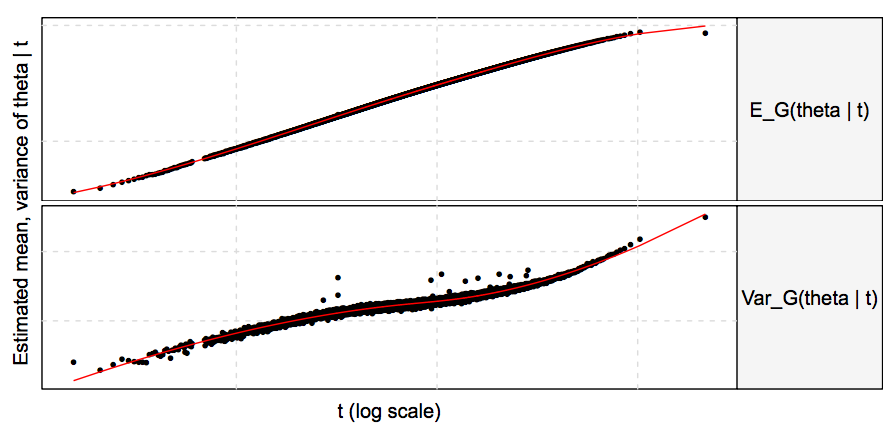 |
| Fig 3: Unsmoothed (dots) and smoothed (red lines) $E G(\theta | t)$ and $\mathrm{var} G(\theta | t)$ (top and bottom, respectively). The former is pretty smooth, but the latter benefits from smoothing. |
We also need to make sure our model fits the data. A simple, necessary check is that the estimated priors lead to marginal distributions that fit the data. This isn’t sufficient, since it doesn’t check our assumed model for the response, $f_\theta$. For example, we might be wrong to assume clicks are Poisson, but a Poisson model could still fit our data with enough freedom in the prior.
One way to check $f_\theta$ is to gather test data and check whether the model fits the relationship between training and test data. This tests the model’s ability to distinguish what is common for each item between the two data sets (the underlying $\theta$) and what is different (the draw from $f_\theta$).
Figure 4 shows the results of such a test. We used our model and training data to construct predictive distributions for test data, and checked where the test data fell in those distributions. If our model were perfect, the test quantiles would be uniform (we jittered the quantiles to account for the discreteness of the data). Our actual quantiles were close to, but not exactly, uniform, indicating a good but not perfect fit.
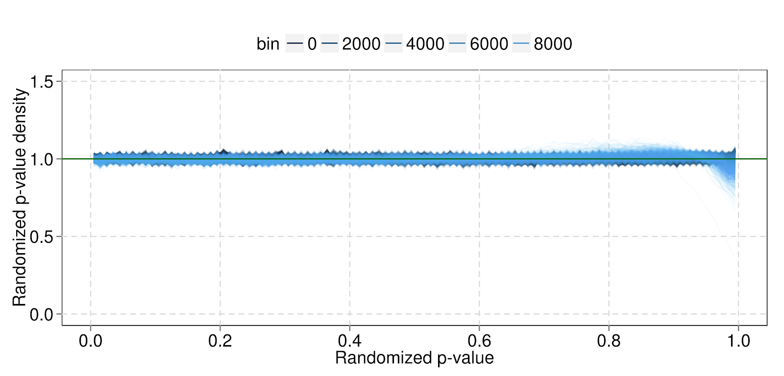 |
| Fig 4: Histograms for the predictive distribution quantiles within each bin, colored by bin. The densities are mostly flat, indicating that our model fits well, but there is some misfit on the right for higher bins. The spikes are artifactual — they appear because we plot the histograms at discrete points, so we see the full range of the curves at those points and not in between. |
Step 4: Posterior quantities
Armed with our validated priors, we can finally calculate interesting posterior quantities. We can’t trust our estimates of every quantity we might be interested in. Standard theory on Empirical Bayes and deconvolution says that we can’t estimate “spiky” functions like $P_G(\theta=0|t,y)$ without additional assumptions. But we can trust our estimates of the first few posterior moments, such as $\mathrm{var}(\theta | t)$, $E(\theta | t, y)$ and $\mathrm{var}(\theta | t, y)$. Each is potentially useful.
$\mathrm{var}(\theta | t)$ is a way to assess accuracy. By comparing $\mathrm{var}(\theta | t)$ to $\mathrm{var}(\theta)$, we can see what fraction of the true variation in $\theta$ is captured by $t$.
$E(\theta | t, y)$ balances memorization and generalization to get an improved estimate of $\theta$. For example, suppose we have a query-ad pair with a single impression ($N = 1$). The empirical CTR for that item will be either 0 or 1, and will tell us almost nothing about the true CTR of that ad. In that case, the best we can do is rely on global information and use $E(\theta | t)$ as our estimate. Conversely, suppose we have a query-ad pair with millions of impressions. The empirical CTR tells us much more about the ad’s true CTR than t does, so we should memorize and use $y/N$ as our estimate. The posterior mean smoothly balances memorization and generalization, depending on the amount of information from each source. Doing this in our calibration instead of just relying on $t$ can be more accurate, and can lead to system simplifications. For example, we could use a relatively coarse generalization model for $t$ and rely on calibration to memorize item-specific information.
$\mathrm{var}(\theta | t, y)$ estimates the accuracy of $E(\theta | t, y)$ — this tells us how much we know about each item. These estimates can be useful to make risk-adjusted decisions and explore-exploit trade-offs, or to find situations where the underlying regression method is particularly good or bad.
Limitations
Second order calibration, like ordinary calibration, is intended to be easy and useful, not comprehensive or optimal, and it shares some of ordinary calibration’s limitations. Both methods can be wrong for slices of the data while being correct on average, since they only use the covariate information through $t$.
Second order calibration also has important additional limitations. We need to know $f_\theta$ to work backwards from the distribution of $y | t$ to that of $\theta | t$. It’s hard to test this assumption directly — a useful indirect check is to make sure the predictive distributions are accurate.
More subtly, second order calibration relies on repeated measurement, in a way that ordinary calibration does not. We must define a unit of observation, and this can be surprisingly tricky. In our CTR example, we defined the unit of observation to be the query-ad pair. But CTR depends on other factors, like the user, and the UI the ad is shown in, and the time of day. It is impossible to refine our unit of observation by all these potential factors and still have repeated measurements for any individual unit. Ordinary calibration and the underlying regression system do not have to solve this problem, since they can just give predictions at the finest-grained level.
We don’t have a fully satisfying answer for this issue. In practice, we have gotten good results by normalizing responses for the first-order effects of factors ignored by our unit definition. More principled solutions could be to account for dispersion within a unit, or to fit some kind of multi-way random effects model.
Conclusion
Second order calibration is a nice example of how dealing with large, complex, changing regression systems requires a different approach. Instead of trying to come up with a principled, correct answer for a particular system, we tried to find something approximate that would work reasonably well without knowing much about the underlying system. The resulting method has clear limitations, but is scalable, maintainable, and accurate enough to be useful.
References
[1] Omkar Muralidharan, Amir Najmi "Second Order Calibration: A Simple Way To Get Approximate Posteriors", Technical Report, Google, 2015.
[2] H. Brendan McMahan et al, "Ad Click Prediction: a View from the Trenches", Proceedings of the 19th ACM SIGKDD International Conference on Knowledge Discovery and Data Mining (KDD), 2013.
[3] Bradley Efron, "Robbins, Empirical Bayes, and Microarrays", Technical Report, 2003.
[4] Bradley Efron, "Large-Scale Inference: Empirical Bayes Methods for Estimation, Testing, and Prediction", Cambridge University Press, 2013.
Comments
Post a Comment