Attributing a deep network’s prediction to its input features
By MUKUND SUNDARARAJAN, ANKUR TALY, QIQI YAN
Editor's note: Causal inference is central to answering questions in science, engineering and business and hence the topic has received particular attention on this blog. Typically, causal inference in data science is framed in probabilistic terms, where there is statistical uncertainty in the outcomes as well as model uncertainty about the true causal mechanism connecting inputs and outputs. And yet even when the relationship between inputs and outputs is fully known and entirely deterministic, causal inference is far from obvious for a complex system. In this post, we explore causal inference in this setting via the problem of attribution in deep networks. This investigation has practical as well as philosophical implications for causal inference. On the other hand, if you just care about understanding what a deep network is doing, this post is for you too.
Deep networks have had remarkable success in variety of tasks. For instance, they identify objects in images, perform language translation, enable web search — all with surprising accuracy. Can we improve our understanding of these methods? Deep networks are the latest instrument in our large toolbox of modeling techniques, and it is natural to wonder about their limits and capabilities. Based on our paper [4], this post is motivated primarily by intellectual curiosity.
Of course, there is benefit to an improved understanding of deep networks beyond the satisfaction of curiosity — developers can use this to debug and improve models; end-users can understand the cause of a model’s prediction, and develop trust in the model. As an example of the latter, suppose that a deep network was used to predict an illness based on an image (from an X-ray, or an MRI, or some other imaging technology). It would be very helpful for a doctor to examine which pixels led to a positive prediction, and cross-check this with her intuition.
We are all familiar with linear and logistic regression models. If we were curious about such a model’s prediction for a given input, we would simply inspect the weights (model coefficients) of the features present in the input. The top few features with the largest weight (i.e., coefficient times feature value) would be indicative of what the model deemed noteworthy.
The goal of this post is to mimic this inspection process for deep models. Can we identify what parts of the input the deep network finds noteworthy? As we soon discuss, the nonlinearity of deep networks makes this problem challenging. The outline of this post is as follows:
Instead, we could use the gradients of the output with respect to the input — if our deep network were linear, this would coincide exactly with the process for linear models, because the gradients correspond to the model coefficients. In effect, we are using a local linear approximation of the (nonlinear) deep network. This approach has been applied to deep networks in previous literature.
Let us see how this does. We are going to inspect the gradient of the score for the object “fireboat” with respect to the input, multiplied point-wise by the input itself (essentially, a Taylor approximation of the prediction function at the input). The result is a matrix that has three dimensions. Two of these correspond to the height and width of the image, and the third is for the primary color (R, G, or B).
Unfortunately, gradients highlight pixels below the bridge which seem completely irrelevant to the “fireboat” prediction. This is unlikely to be a model bug — recall that the prediction was correct. So what is happening?
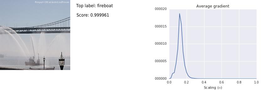
It turns out that our local linear approximation does a poor job of indicating what the network thinks is important. The prediction function flattens in the vicinity of the input, and consequently, the gradient of the prediction function with respect to the input is tiny in the vicinity of the input vector. The dot product of the gradient with the image, which represents a first-order Taylor approximation of the prediction function at the input, adds up to only $4.6 \times 10^{-5}$ (while the actual value of the prediction is $0.999961$ — gradients aren’t accounting for a large portion of the score.
A simple analysis substantiates this. We construct a series of images by scaling down the pixel intensities from the actual image to zero (black). Call this scaling parameter $\alpha$. One can see that the prediction function flattens after $\alpha$ crosses $0.2$.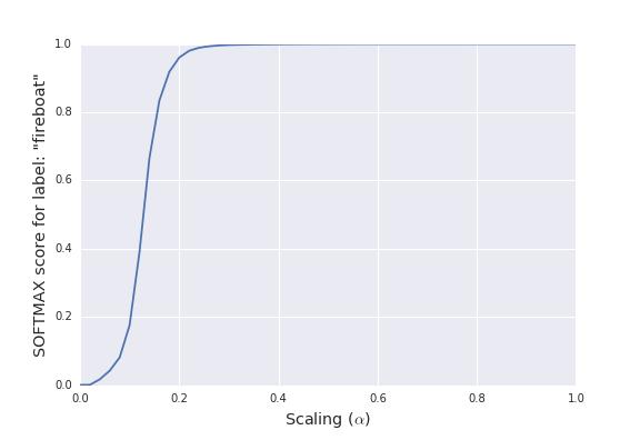
This phenomenon of flattening is specific neither to this label (“fireboat”), this image, the output neuron, or nor even to this network. It has been observed by other work [2] and our previous paper [3].
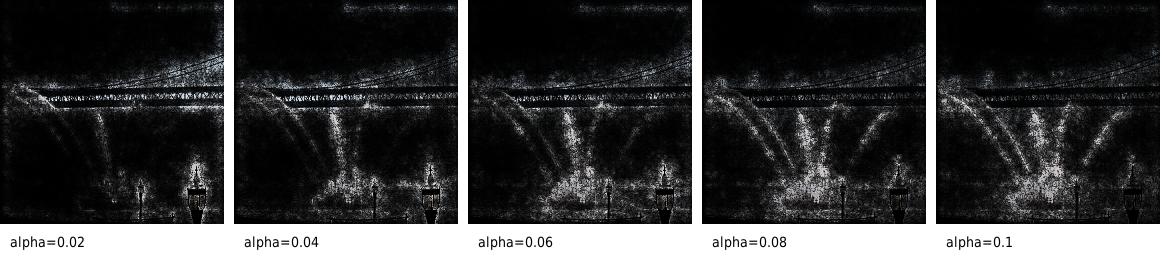
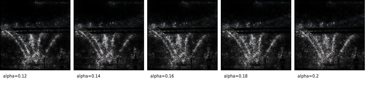
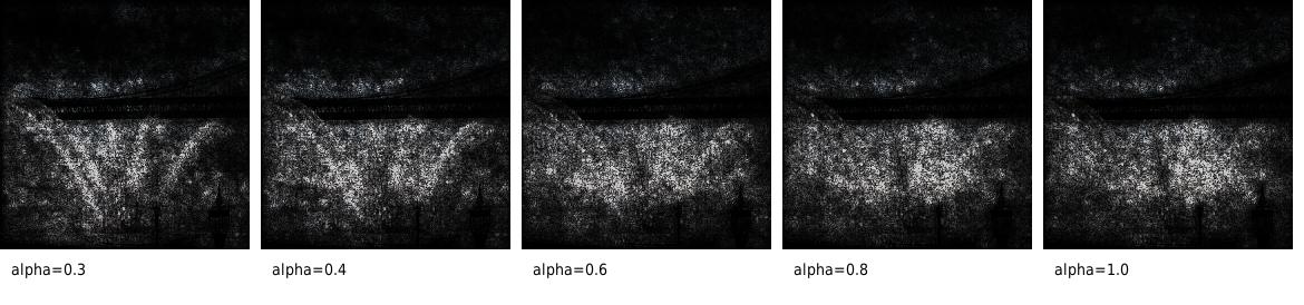
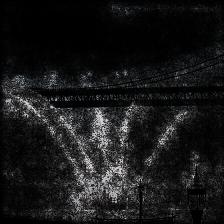
The visualizations show that at lower values of the scaling parameter $\alpha$, the pixels constituting the fireboat and spout of water are most important. But as $\alpha$ increases, the region around the fireboat (rather than the fireboat itself) gains relative importance. As the plot shows, the visualizations corresponding to lower values of the scale parameter are more important to the score because they have higher gradient magnitudes. This does not come through in our visualizations because they are each normalized for brightness; if they weren’t, the last few images would look nearly black. By summing the gradients across the images, and then visualizing this, we get a more realistic picture of what is going on.
This is the essence of our method. We call this method "integrated gradients". Informally, we average the gradients of the set of scaled images and then take the element-wise product of this with the original image. Formally, this approximates a certain integral as we will see later.
The complete code for loading the Inception model and visualizing the attributions is available from GitHub repository. The code is packaged as a single IPython notebook with less than 70 lines of Python TensorFlow code. Instructions for running the notebook are provided in our README. Below is the key method for generating integrated gradients for a given image and label. It involves scaling the image and invoking the gradient operation on the scaled images:
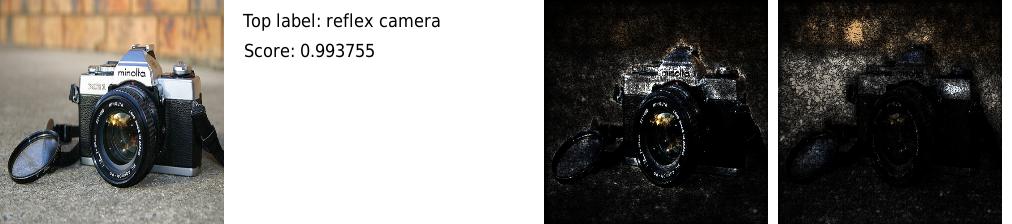
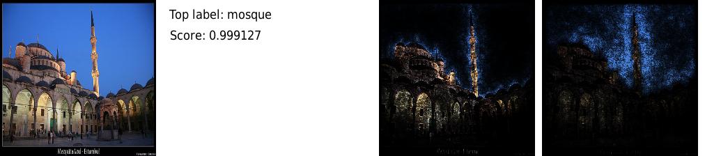
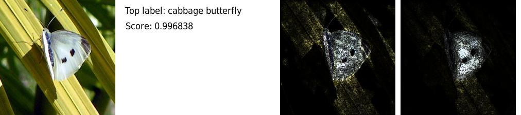
The following figure shows some more visualizations of integrated gradients. Our visualization logic is identical to that of the gradient approach. For comparison, we also show the visualization for the gradient approach. From the visualizations, it is evident that the integrated gradients are better at capturing important features.


In our ImageNet example, the function $F$ represents the Inception deep network (for a given output class). The input vector $x$ is simply the image — if one represents the image in grayscale, the indices of $x$ correspond to the pixels. The attribution vector $a$ is exactly what we visualize in the previous sections.
Let us briefly examine the need for the baseline in the definition of the attribution problem. A common way for humans to perform attribution relies on counterfactual intuition. When we assign blame to a certain cause we implicitly consider the absence of the cause as a baseline — would the outcome change if the supposed cause were not present?
The attribution scheme for linear models that inspects the weights of the input features has an implicit baseline of an input with no features. The gradient based approach uses a baseline that is a slight perturbation of the original input. Of course, gradients, as we argued earlier, are a poor attribution scheme. Intuitively, the baseline is “too close” to the input. For integrated gradients, we will use baselines that are far enough away from the input that they don’t just focus on the flat region in the sense of the saturation plot shown in the earlier section. We will also ensure that baseline is fairly “neutral”, i.e., the predictions for this input are nearly zero. For instance, the black image for an object recognition network. This will allow us to interpret the attributions independent of the baseline as a property of the input alone.
Completeness: The attributions from integrated gradients sum to the difference between the prediction scores of the input and the baseline. The proof follows from the famous gradient theorem. This property is desirable because we can be sure that the prediction is entirely accounted for.
Linearity preservation: If a network $F$ is a linear combination $a*F_1 + b*F_2$ of two networks $F_1$ and $F_2$, then a linear combination of the attributions for $F_1$ and $F_2$, with weights $a$ and $b$ respectively, is the attribution for the network $F$. The property is desirable because the attribution method preserves any linear logic present within a network.
Symmetry preservation: Integrated gradients preserve symmetry. That is, if the network behaves symmetrically with respect to two input features, then the attributions are symmetric as well. For instance, suppose $F$ is a function of three variables $x_1, x_2, x_3$, and $F(x_1,x_2, x_3) = F(x_2,x_1, x_3)$ for all values of $x_1, x_2, x_3$. Then $F$ is symmetric in the two variables $x_1$ and $x_2$. If the variables have identical values in the input and baseline, i.e., $x_1 = x_2$, and $x'_1 =x'_2$, then symmetry preservation requires that $a_1 = a_2$. This property seems desirable because of the connotation of attributions as blame assignment. Why should two symmetric variables be blamed differently?
Sensitivity: We define two aspects of sensitivity.
At first glance, these requirements above seem quite basic and we may expect that many methods ought to provably satisfy them. Unfortunately, other methods in literature fall into classes — they either violate Sensitivity(A) or they violate an even more basic property, namely they depend on the implementation of the network in an undesirable way. That is, we can find examples where two networks have identical input-output behavior, but the method yields different attributions (due to a difference in the underlying structure of the two networks). In contrast, our method relies only on the functional representation of the network, and not its implementation, i.e., we say that it satisfies "implementation invariance".
In contrast, we can show that our method is essentially the unique method to satisfy all the properties listed above (up to certain convex combinations). We invite the interested reader to read our paper [4], where we have formal descriptions of these properties, the uniqueness result, and comparisons with other methods.
A quick checklist on applying our method to your favorite deep network. You will have to resolve three issues:
Of course, our problem formulation has limitations. It says nothing about the logic that is employed by the network to combine features. This is an interesting direction for future work.
Our method and our problem statement are also restricted to providing insight into the behavior of the network on a single input. It does not directly offer any global understanding of the network. Other work has made progress in this direction via clustering inputs using the pattern of neuron activations, for instance, [5] or [6]. There is also work (such as this) on architecting deep networks in ways that allow us to understand the internal representations of these networks. These are all very insightful. It is interesting to ask if there is a way to turn these insights into guarantees of some form as we do for the problem of feature attribution.
Overall, we hope that deep networks lose their reputation for being impenetrable black-boxes which perform black magic. Though they are harder to debug than other models, there are ways to analyze them. And the process can be enlightening and fun!
[2] Shrikumar, Avanti, Greenside, Peyton, Shcherbina, Anna, and Kundaje, Anshul. Not just a black box: Learning important features through propagating activation differences. CoRR, 2016.
[3] Mukund Sundararajan, Ankur Taly, Qiqi Yan, 2016, "Gradients of Counterfactuals", arXiv:1611.02639
[4] Mukund Sundararajan, Ankur Taly, Qiqi Yan, 2017, "Axiomatic Attribution for Deep Networks", arXiv:1703.01365
[5] Ian J. Goodfellow, Quoc V. Le, Andrew M. Saxe, Honglak Lee, and Andrew Y. Ng. 2009, "Measuring invariances in deep networks". In Proceedings of the 22nd International Conference on Neural Information Processing Systems (NIPS'09), USA, 646-654
Deep networks have had remarkable success in variety of tasks. For instance, they identify objects in images, perform language translation, enable web search — all with surprising accuracy. Can we improve our understanding of these methods? Deep networks are the latest instrument in our large toolbox of modeling techniques, and it is natural to wonder about their limits and capabilities. Based on our paper [4], this post is motivated primarily by intellectual curiosity.
Of course, there is benefit to an improved understanding of deep networks beyond the satisfaction of curiosity — developers can use this to debug and improve models; end-users can understand the cause of a model’s prediction, and develop trust in the model. As an example of the latter, suppose that a deep network was used to predict an illness based on an image (from an X-ray, or an MRI, or some other imaging technology). It would be very helpful for a doctor to examine which pixels led to a positive prediction, and cross-check this with her intuition.
We are all familiar with linear and logistic regression models. If we were curious about such a model’s prediction for a given input, we would simply inspect the weights (model coefficients) of the features present in the input. The top few features with the largest weight (i.e., coefficient times feature value) would be indicative of what the model deemed noteworthy.
The goal of this post is to mimic this inspection process for deep models. Can we identify what parts of the input the deep network finds noteworthy? As we soon discuss, the nonlinearity of deep networks makes this problem challenging. The outline of this post is as follows:
- we introduce a natural approach to attribution based on gradients
- use failures of the gradient approach to guide the design of our method
- present our method more formally and discuss its properties
- describe applications to networks other than Inception/ImageNet (our running example)
We conclude with some areas for future work.
Feature Importance via Gradients
Feature attribution for (generalized) linear models
Suppose that our model is linear. Then, there is a simple, commonly followed practice to identify the importance of features — examine the coefficients of the features present in the input, weighted by the values of these features in the input. (One can think of categorical features as having values in $\{0,1\}$.) A summation of the resulting vector would equal the prediction score less the intercept term and so this process accounts for the entire prediction. If instead of summing, we sorted this vector in decreasing sequence of magnitude, we would identify the features that the model finds important. Occasionally, we may find that the coefficients don’t match our intuition of what is important. We may then check for overfitting, or for biases in the training data, and fix these issues. Or we find may that some of the features are correlated, and the strange coefficients are an artifact thereof. In either case, this process is integral to improving the network or trusting its prediction. Let us now attempt to mimic this process for deep networks.The Inception architecture and ImageNet
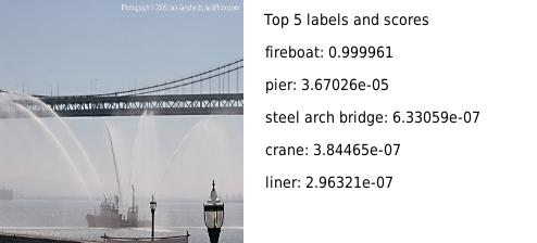
For concreteness, let us focus on a network that performs object recognition. We consider a deep network using the Inception [1] architecture trained on the ImageNet dataset. It takes an image as input and assigns scores for 1000 different ImageNet categories. The input is specified via the R,G,B values of the pixels of the image. At the output, the network produces a score (probability) for each label using a multinomial logit (Softmax) function. The network “thinks” that objects with large output scores are probably present in the image. For instance, here is an image and its top few labels:
Notice that the score for the top label, “fireboat”, is very close to 1.0, indicating that the network is very sure that there is a “fireboat” somewhere in the image. The network is absolutely right in this case — a fireboat is a special boat used to fight fires on shorelines and aboard ships.
Applying Gradients to Inception
Which pixels made the network think of this as a fireboat? We cannot just examine the coefficients of the model as we do with linear models. Deep networks have multiple layers of logic and coefficients, combined using nonlinear activation functions. For instance, the Inception architecture has 22 layers. The coefficients of the input layer do not adequately cover the logic of the network. In contrast, the coefficients of the hidden layers aren’t in any human intelligible space.Instead, we could use the gradients of the output with respect to the input — if our deep network were linear, this would coincide exactly with the process for linear models, because the gradients correspond to the model coefficients. In effect, we are using a local linear approximation of the (nonlinear) deep network. This approach has been applied to deep networks in previous literature.
Let us see how this does. We are going to inspect the gradient of the score for the object “fireboat” with respect to the input, multiplied point-wise by the input itself (essentially, a Taylor approximation of the prediction function at the input). The result is a matrix that has three dimensions. Two of these correspond to the height and width of the image, and the third is for the primary color (R, G, or B).
A note on visualization
The most convenient way to inspect our feature importances (attributions) is to visualize them. We do this by using the attributions as a (soft) window over the image itself. We construct the window by first removing the primary color dimension from the attributions, by taking the sum of absolute value of the R, G, B values. To window the image, we take an element-wise product of the window with the pixel values and visualize the resulting image. The result is that unimportant pixels are dimmed. Our code has details (there are probably other reasonable visualization approaches that work just as well). The visualization of the gradients for the “fireboat” image looks like this:Unfortunately, gradients highlight pixels below the bridge which seem completely irrelevant to the “fireboat” prediction. This is unlikely to be a model bug — recall that the prediction was correct. So what is happening?
It turns out that our local linear approximation does a poor job of indicating what the network thinks is important. The prediction function flattens in the vicinity of the input, and consequently, the gradient of the prediction function with respect to the input is tiny in the vicinity of the input vector. The dot product of the gradient with the image, which represents a first-order Taylor approximation of the prediction function at the input, adds up to only $4.6 \times 10^{-5}$ (while the actual value of the prediction is $0.999961$ — gradients aren’t accounting for a large portion of the score.
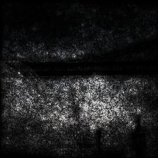
A simple analysis substantiates this. We construct a series of images by scaling down the pixel intensities from the actual image to zero (black). Call this scaling parameter $\alpha$. One can see that the prediction function flattens after $\alpha$ crosses $0.2$.
This phenomenon of flattening is specific neither to this label (“fireboat”), this image, the output neuron, or nor even to this network. It has been observed by other work [2] and our previous paper [3].
Our method: Integrated Gradients
The same plot that demonstrates why gradients don’t work also tells us how to fix the issue. Notice that there is a large jump in the prediction score at low intensities. Perhaps it is useful to inspect the gradients of those images. The figure below visualizes these gradients, visualized with the same logic as in the previous section; these are just the gradients of the original image at different levels of brightness.The visualizations show that at lower values of the scaling parameter $\alpha$, the pixels constituting the fireboat and spout of water are most important. But as $\alpha$ increases, the region around the fireboat (rather than the fireboat itself) gains relative importance. As the plot shows, the visualizations corresponding to lower values of the scale parameter are more important to the score because they have higher gradient magnitudes. This does not come through in our visualizations because they are each normalized for brightness; if they weren’t, the last few images would look nearly black. By summing the gradients across the images, and then visualizing this, we get a more realistic picture of what is going on.
This is the essence of our method. We call this method "integrated gradients". Informally, we average the gradients of the set of scaled images and then take the element-wise product of this with the original image. Formally, this approximates a certain integral as we will see later.
The complete code for loading the Inception model and visualizing the attributions is available from GitHub repository. The code is packaged as a single IPython notebook with less than 70 lines of Python TensorFlow code. Instructions for running the notebook are provided in our README. Below is the key method for generating integrated gradients for a given image and label. It involves scaling the image and invoking the gradient operation on the scaled images:
def integrated_gradients(img, label, steps=50):
'''Returns attributions for the prediction label based
on integrated gradients at the image.
Specifically, the method returns the dot product of the image
and the average of the gradients of the prediction label (w.r.t.
the image) at uniformly spaced scalings of the provided image.
The provided image must of shape (224, 224, 3), which is
also the shape of the returned attributions tensor.
'''
# Obtain the tensor representing the softmax output of the provided label.
t_output = output_label_tensor(label) # shape: scalar
t_grad = tf.gradients(t_output, T('input'))[0]
scaled_images = [(float(i)/steps)*img for i in range(1, steps+1)]
# Compute the gradients of the scaled images
grads = run_network(sess, t_grad, scaled_images)
# Average the gradients of the scaled images and dot product with the original
# image
return img*np.average(grads, axis=0)
Misclassifications
We now turn to images that are misclassified by the Inception network, i.e., where the top five labels assigned by the Inception network are different from the ground truth label provided by the ImageNet dataset. The goal is understand what made the network choose the wrong label? To understand this we visualize the integrated gradients with respect to the top label assigned by the Inception network (i.e., the wrong label).

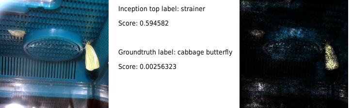
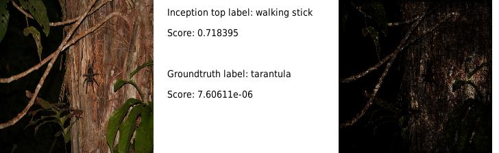
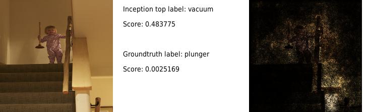
With the first image, it is clear what went wrong even without examining the integrated gradients. The image does have a strainer, but the ground truth label is about a different object within the image (cabbage butterfly). In contrast, the second and third images are more mysterious. Inspecting the images alone do not tell us anything about the source of the error. The integrated gradient visualization is clarifying — it identifies blurry shapes within the image that seem to resemble a walking stick and a vacuum cleaner. Perhaps a fix for these misclassifications is to feed these images as negative examples for the incorrect labels.
With the first image, it is clear what went wrong even without examining the integrated gradients. The image does have a strainer, but the ground truth label is about a different object within the image (cabbage butterfly). In contrast, the second and third images are more mysterious. Inspecting the images alone do not tell us anything about the source of the error. The integrated gradient visualization is clarifying — it identifies blurry shapes within the image that seem to resemble a walking stick and a vacuum cleaner. Perhaps a fix for these misclassifications is to feed these images as negative examples for the incorrect labels.
Properties of Integrated Gradients
We use this section to be precise about our problem statement, our method, and its properties. Part of the reason for the rigor is to argue why our method does not introduce artifacts into the attributions, and faithfully reflects the workings of the deep network.Attribution Problem
Formally, suppose we have a function $F: \mathbb{R}^n \rightarrow [0,1]$ that represents a deep network, and an input $x = (x_1,\ldots,x_n) \in \mathbb{R}^n$. An attribution of the prediction at input $x$ relative to a baseline input $x'$ is a vector $A_F(x, x') = (a_1,\ldots,a_n) \in \mathbb{R}^n$ where $a_i$ is the contribution of $x_i$ to the function $F(x)$.
In our ImageNet example, the function $F$ represents the Inception deep network (for a given output class). The input vector $x$ is simply the image — if one represents the image in grayscale, the indices of $x$ correspond to the pixels. The attribution vector $a$ is exactly what we visualize in the previous sections.
Let us briefly examine the need for the baseline in the definition of the attribution problem. A common way for humans to perform attribution relies on counterfactual intuition. When we assign blame to a certain cause we implicitly consider the absence of the cause as a baseline — would the outcome change if the supposed cause were not present?
The attribution scheme for linear models that inspects the weights of the input features has an implicit baseline of an input with no features. The gradient based approach uses a baseline that is a slight perturbation of the original input. Of course, gradients, as we argued earlier, are a poor attribution scheme. Intuitively, the baseline is “too close” to the input. For integrated gradients, we will use baselines that are far enough away from the input that they don’t just focus on the flat region in the sense of the saturation plot shown in the earlier section. We will also ensure that baseline is fairly “neutral”, i.e., the predictions for this input are nearly zero. For instance, the black image for an object recognition network. This will allow us to interpret the attributions independent of the baseline as a property of the input alone.
Integrated Gradients
We are now ready to define our method formally. The integrated gradient along the $i^{th}$ dimension for an input $x$ and baseline $x'$ is defined as follows:
$$
\mathrm{IntegratedGrads}_i(x) ::= (x-x')\times\int_{\alpha=0}^{1}
\frac{\partial F(x' + \alpha \times(x-x'))}{\partial x_i
}~d\alpha
$$
\mathrm{IntegratedGrads}_i(x) ::= (x-x')\times\int_{\alpha=0}^{1}
\frac{\partial F(x' + \alpha \times(x-x'))}{\partial x_i
}~d\alpha
$$
where $\frac{\partial F(x)}{\partial x_i}$ is the gradient of $F$ along the $i^{th}$ dimension at $x$.
Below we list a number of properties that our method satisfies:
Completeness: The attributions from integrated gradients sum to the difference between the prediction scores of the input and the baseline. The proof follows from the famous gradient theorem. This property is desirable because we can be sure that the prediction is entirely accounted for.
Linearity preservation: If a network $F$ is a linear combination $a*F_1 + b*F_2$ of two networks $F_1$ and $F_2$, then a linear combination of the attributions for $F_1$ and $F_2$, with weights $a$ and $b$ respectively, is the attribution for the network $F$. The property is desirable because the attribution method preserves any linear logic present within a network.
Symmetry preservation: Integrated gradients preserve symmetry. That is, if the network behaves symmetrically with respect to two input features, then the attributions are symmetric as well. For instance, suppose $F$ is a function of three variables $x_1, x_2, x_3$, and $F(x_1,x_2, x_3) = F(x_2,x_1, x_3)$ for all values of $x_1, x_2, x_3$. Then $F$ is symmetric in the two variables $x_1$ and $x_2$. If the variables have identical values in the input and baseline, i.e., $x_1 = x_2$, and $x'_1 =x'_2$, then symmetry preservation requires that $a_1 = a_2$. This property seems desirable because of the connotation of attributions as blame assignment. Why should two symmetric variables be blamed differently?
Sensitivity: We define two aspects of sensitivity.
- (A) If the baseline and the input differ only in one feature, but have different predictions, then this feature gets non-zero attribution.
- (B) If a feature does not play any role in the network, it receives no attributions.
At first glance, these requirements above seem quite basic and we may expect that many methods ought to provably satisfy them. Unfortunately, other methods in literature fall into classes — they either violate Sensitivity(A) or they violate an even more basic property, namely they depend on the implementation of the network in an undesirable way. That is, we can find examples where two networks have identical input-output behavior, but the method yields different attributions (due to a difference in the underlying structure of the two networks). In contrast, our method relies only on the functional representation of the network, and not its implementation, i.e., we say that it satisfies "implementation invariance".
In contrast, we can show that our method is essentially the unique method to satisfy all the properties listed above (up to certain convex combinations). We invite the interested reader to read our paper [4], where we have formal descriptions of these properties, the uniqueness result, and comparisons with other methods.
Application to other networks
Our paper also includes application of integrated gradients to other networks (none of these networks were trained by us). One network is an image network that predicts diabetic retinopathy — we demonstrate the use of attributions in a user-facing context to help doctors gain some transparency into the network’s prediction. The second network is a chemistry network that performs virtual screening of drug molecules — we show how attributions help identify degenerate model features. A third network categorizes queries in the context of a question-answering system — we demonstrate the use of attribution to extract human-intelligible rules.A quick checklist on applying our method to your favorite deep network. You will have to resolve three issues:
- Identify a good baseline, i.e., the analog of the black image in our example. This should be treated as neutral by the network, i.e., the prediction score for this input should be nearly zero.
- Identify the right variables to attribute to. This step is trivial for ImageNet. But in a text network the input is usually represented as embeddings. The attributions are then naturally produced in the space of embeddings and some simple processing is needed to map them to the space of terms.
- Find a convenient visualization technique. Our paper [4] has some ideas.
Concluding thoughts
This post discusses the problem of identifying input feature importance for a deep network. We present a very simple method, called "integrated gradients", to do this. All it involves is a few calls to a gradient operator. It yields insightful results for a variety of deep networks.Of course, our problem formulation has limitations. It says nothing about the logic that is employed by the network to combine features. This is an interesting direction for future work.
Our method and our problem statement are also restricted to providing insight into the behavior of the network on a single input. It does not directly offer any global understanding of the network. Other work has made progress in this direction via clustering inputs using the pattern of neuron activations, for instance, [5] or [6]. There is also work (such as this) on architecting deep networks in ways that allow us to understand the internal representations of these networks. These are all very insightful. It is interesting to ask if there is a way to turn these insights into guarantees of some form as we do for the problem of feature attribution.
Overall, we hope that deep networks lose their reputation for being impenetrable black-boxes which perform black magic. Though they are harder to debug than other models, there are ways to analyze them. And the process can be enlightening and fun!
References
[1] Szegedy, Christian, Liu, Wei, Jia, Yangqing, Sermanet,
Pierre, Reed, Scott E., Anguelov, Dragomir, Erhan, Dumitru,
Vanhoucke, Vincent, and Rabinovich, Andrew.
Going deeper with convolutions. CoRR, 2014.
[2] Shrikumar, Avanti, Greenside, Peyton, Shcherbina, Anna, and Kundaje, Anshul. Not just a black box: Learning important features through propagating activation differences. CoRR, 2016.
[4] Mukund Sundararajan, Ankur Taly, Qiqi Yan, 2017, "Axiomatic Attribution for Deep Networks", arXiv:1703.01365
[5] Ian J. Goodfellow, Quoc V. Le, Andrew M. Saxe, Honglak Lee, and Andrew Y. Ng. 2009, "Measuring invariances in deep networks". In Proceedings of the 22nd International Conference on Neural Information Processing Systems (NIPS'09), USA, 646-654
[6] Erhan, Dumitru, Bengio, Yoshua, Courville, Aaron, and
Vincent, Pascal. "Visualizing higher-layer features of a deep network". Technical Report 1341, University of
Montreal, 2009.
Hello! I came across this while studying for an interview at google and this concept seems very interesting to me. I know highly regulated fields like in risk management and medicine ("old fashioned statistic") are adverse to using neural networking models because they currently are unexplainable in terms of the feature space. Defining metrics like these could go a long way in changing hearts and minds!
ReplyDeleteA few constructive feedback pieces I would like to offer if it helps:
1) Although noise might be considered meaningless here if the data is large enough, it would be useful to see how your metric infers confidence bounds on neural networks. Particularly, I would love to see if this constructs a GLM "p-value" of sorts which can gauge the probability that at least the function has a critical point at x_0.
2) By assuming the function has a gradient it seems you aren't entirely adverse to believing the function is smooth. If I were designing this I think I would have come up with something similar actually except I would have used the absolute value of the partial derivative. Reason being that as I think the neural network is an analytic function (in its classical construction it is a finite composition of sigmoid functions) and showing an analytic function is zero uniformly on any closed curve implies it is zero on the interior. Have you considered this approach?
Dear dp1080,
DeleteI'd love to have a more detailed chat about what you mean with the stokes theorem references and also the p-value point. It sounds interesting, but I am not able to unpack all of it. Could we chat over mail (mukunds@google.com)?
I am happy to update this blog post with a summary of our chat.
(1. we have played with absolute values in the past
2. ReLU based networks provably satisfy the degree of smoothness we need to run our method.)
thanks!
It seems that if one has a more traditional supervised learning problem with a set of features and either numeric or categorical response, this method does not work?
ReplyDelete