Our quest for robust time series forecasting at scale
by ERIC TASSONE, FARZAN ROHANI
We were part of a team of data scientists in Search Infrastructure at Google that took on the task of developing robust and automatic large-scale time series forecasting for our organization. In this post, we recount how we approached the task, describing initial stakeholder needs, the business and engineering contexts in which the challenge arose, and theoretical and pragmatic choices we made to implement our solution.
In terms of scope, we sought to forecast a large number of time series, and to do so frequently. We wanted to forecast a variety of quantities: overall search query volume and particular types of queries; revenue; views and minutes of video watched on Google-owned YouTube (which recently reached a billion hours daily); usage of sundry internal resources; and more. Additionally, we often had an independent interest in subseries of those quantities, such as disaggregated by locale (e.g., into >100 countries or regions), device type (e.g., by desktop, mobile, and tablet), and operating system, as well as combinations of all these (e.g., locale-by-device type.) Given the assortment of quantities and their combinatorial explosion into subseries, our forecasting task was easily on the order of tens of thousands of forecasts. And then we wanted to forecast these quantities every week, or in some cases more often.
The variety and frequency of forecasts demanded robust, automatic methods --- robust in the sense of dramatically reducing the chance of a poor forecast regardless of the particular characteristics of the time series being forecast (e.g., its growth profile) and automatic in the sense of not requiring human intervention before or after running the forecast.
Another important domain constraint was that our time series were the result of some aggregate human phenomenon --- search queries, YouTube videos viewed, or (as in our example) electricity consumed in Turkey. Unlike physical phenomena such as earthquakes or the tides, the time series we forecast are shaped by the rhythms of human civilization and its weekly, annual, and at-times irregular and evolving cycles. Calendaring was therefore an explicit feature of models within our framework, and we made considerable investment in maintaining detailed regional calendars.
Our initial use case did not involve explanatory variables, instead relying only the time series histories of the variables being forecast. Our rationale was in accord with the views expressed in the online forecasting book by Hyndman and Athanasopoulos [1], who after mentioning the potential utility of an "explanatory model" write:
However, there are several reasons a forecaster might select a time series model rather than an explanatory model. First, the system may not be understood, and even if it was understood it may be extremely difficult to measure the relationships that are assumed to govern its behavior. Second, it is necessary to know or forecast the various predictors in order to be able to forecast the variable of interest, and this may be too difficult. Third, the main concern may be only to predict what will happen, not to know why it happens. Finally, the time series model may give more accurate forecasts than an explanatory or mixed model.
"Forecasting" for us also did not mean using time series in a causal inference setting. There are tools for this use case, such as Google-supported CausalImpact.
CausalImpact is powered by bsts (“Bayesian Structural Time Series”), also from Google, which is a time series regression framework using dynamic linear models fit using Markov chain Monte Carlo techniques. The regression-based bsts framework can handle predictor variables, in contrast to our approach. Facebook in a recent blog post unveiled Prophet, which is also a regression-based forecasting tool. But like our approach, Prophet aims to be an automatic, robust forecasting tool.
At lastly, "forecasting" for us did not mean anomaly detection. Tools such as Twitter’s AnomalyDetection or RAD ("Robust Anomaly Detection") from Netflix, as their names suggest, target this type of problem.
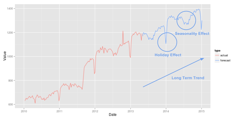
Missing values and putative anomalous values may present as a dramatic spike or drop not explained by a launch, seasonality effect, or holiday impact. They can arise from data collection errors or other unlikely-to-repeat causes such as an outage somewhere on the Internet. If unaccounted for, these data points can have an adverse impact on forecast accuracy by disrupting seasonality, holiday, or trend estimation.
Level changes are different in that they represent a more permanent change in the level of the time series, in contrast to anomalies, where the time series returns to its previous level at trend after a brief period. They may result from launches, logging changes, or external events. At a minimum, adjusting for level changes results in a longer effective time series, and often makes trend estimation easier when the models are finally fit.
We also permit transformations, such as a Box-Cox transformation. These can be automatic (the default setting for some models) or user-specified. These too can help with meeting model assumptions and with eventual forecast accuracy (final forecasts must be re-transformed to the original scale, of course).
For the effect adjustments we seek to: quantify the effect; remove the effect from the time series; forecast the time series without the effect; and re-apply the effect to that forecast post hoc. By contrast, for cleaning adjustments, we seek only to quantify, so as to remove. In addition, for the effect adjustments, we typically have business-knowledge or day-to-day-operations motivations for wanting to know the magnitude of the effect; this is not always the case for cleaning adjustments.
Though not cleanly separated conceptually, holiday effects and seasonality effects are partially distinguished in that seasonality effects are defined as occurring during the same numerical week of the year, whereas holiday effects are specific to the day of the occurrence and adjacent "shoulder" days. That said, some holidays fall on the same calendar day but on a different day of the week each year, such as Independence Day falling on the 4th of July in the United States; some fall on the same day of the week and week of the year, but on a different calendar day, such as Thanksgiving Day falling on the fourth Thursday of November in the United States; and some vary with solar or lunar phenomena, such as the Easter Sunday holiday celebrated in many countries around the world, which can fall anywhere from late March to late April. Due to these differences, some holiday effects and seasonality effects may not be identifiable. But note the use of "week" as the germane unit of time for seasonality and "day" for holidays: We estimate holiday effects from the adjusted daily data, but then roll up daily values to weekly totals before estimating seasonality effects.
Estimating holiday and seasonality effects is more art than science due to the paucity of relevant historical data. For instance, to estimate the effect of Independence Day when it falls on a weekday versus a weekend, you can accrue observations only so fast! And the effect may evolve as, say, smart phones proliferate and people begin doing more Google Maps searches the evening of Independence Day. Our experience with holiday adjustments is that ad hoc methods which work well and are easily interpretable (if only for debugging) are preferred to elegant, comprehensive mathematical models which may not deliver nor are amenable to a postmortem when something (inevitably) goes wrong.
The plots below illustrate a toy example of cleaning and effects adjustments in action. In the first plot, the raw weekly actuals (in red) are adjusted for a level change in September 2011 and an anomalous spike near October 2012. The cleaned weekly actuals (in green) are much smoother, but still show strong seasonal and holiday effects. As noted above, these are estimated, removed, the long-term trend is forecast, and then the seasonal and holiday effects are added back, producing the weekly forecast (in blue), as shown in the second plot.

In our experience there are great dividends in treating the forecasting task, with its priority on growth trend estimation, separately from the day-of-week effect. By decomposing the overall problem, we can focus on methods that best solve the specific subproblem. For us, forecasting the trend from less noisy weekly data (again, and importantly, after cleaning and effect adjustments) results in better growth trend estimation compared to all-in-one methods. Methods that attempt to simultaneously estimate all relevant parameters in a unified framework may be vulnerable to omission, overfitting, confounding of effects, or something else going awry which subsequently impairs the method's ability to accurately estimate the growth trend.
Likewise, by treating the day-of-week effect on its own we can deploy methods targeted to capturing its important aspects. For instance, in our data we often see secular trends as well as annual seasonality in the amplitude of the weekly cycle i.e., long-term changes to the proportions of the weekly total going to each day of the week and intra-year cycles in these proportions. A model general enough to accommodate such phenomena, and everything else, along with the data to identify all relevant parameters is for us too much to ask. Such a model risks conflating important aspects, notably the growth trend, with other less critical aspects.
Consider, for example, Global search queries. The first step, disaggregation, is quite natural. Search queries are logged with many attributes, and we typically use at least geography and device type. This aspect is easy. Next, forecasting the many subseries: Again, this is easy --- our forecast methodology is designed to be robust and automatic, so dramatically increasing the number of forecasts is not overly risky, either. Lastly, however, we need a method to take this collection of forecasts and reconcile them. This is more challenging.
A simple solution is to forecast only at the bottom of the hierarchy and simply sum the forecasts to produce an overall parent forecast (and indeed forecasts all throughout the hierarchy.) This can be quite effective, as the important differences in growth profiles tend to arise across the geography-by-device-type boundaries, and forecasting them independently as a first step frees them.
An obvious requisite property of reconciliation is arithmetic coherence across the hierarchy (which is implicit in the sum-up-from-the-bottom possibility in the previous paragraph), but more sophisticated reconciliation may induce statistical stability of the constituent forecasts and improve forecast accuracy across the hierarchy. While we use reconciliation methods tailored to our specific context, similar techniques have been implemented in the R package hts and written about in the literature.
Though more sophisticated, more mathematically alluring options are available for producing a final forecast from an ensemble, such as Bayesian Model Averaging, we opt for simple approaches. The confluence of our beliefs about the world, underlying theoretical results, and empirical performance compel us toward deriving a final forecast from the ensemble via a simple measure of central tendency (i.e., a mean or median) after some effort to remove outliers (which could be as simple as trimming or winsorizing.) Crucially, our approach does not rely on model performance on holdout samples. Details follow, but first an exploration of why such an embarrassingly simple and seemingly ad hoc approach might do so well in this setting.
In many studies, the average of the individual forecasts has performed best or almost best. Statisticians interested in modeling forecasting systems may find this state of affairs frustrating. The questions that need to be answered are (1) why does the simple average work so well, and (2) under what conditions do other specific methods work better?
Clemen then homes in on a contradiction inherent in the pursuit of sophisticated combination strategies (emphasis added):
From a conventional forecasting point of view, using a combination of forecasts amounts to an admission that the forecaster is unable to build a properly specified model. Trying ever more elaborate combining models seems only to add insult of injury, as the more complicated combinations do not generally perform all that well.
With that context, consider an example inspired by Bates and Granger [4] and by [3]. Define two independent random variables $X_1 \sim N(0, 1)$ and $X_2 \sim N(0, 2)$. For this simple vignette, we might regard $X_1$ and $X_2$ as errors from a measuring scale and note that $X_2$ is not as precise an instrument as $X_1$. Define
However, consider another scenario. Suppose $X_1$ and $X_2$ are independent as before, but now suppose we only know that one of $X_1$ and $X_2$ is distributed as $N(0, 1)$ and the other as $N(0, 2)$, and we do not know which is which. Thus with equal chance we might have $X_1 \sim N(0, 1)$ and $X_2 \sim N(0, 2)$ or $X_1 \sim N(0, 2)$ and $X_2 \sim N(0, 1)$. Let’s again form $X_A$ and $X_C$ as before. $X_A$ is unchanged, regardless of how $X_1$ and $X_2$ are actually distributed, with $X_A \sim N(0, \frac{3}{4})$. If $X_1$ has the lower variance we once again have $X_C \sim N(0, \frac{2}{3})$. But if it is the case that $X_1 \sim N(0, 2)$ and $X_2 \sim N(0, 1)$, then the variance of $X_C$ would be $1$. This would be an inferior instrument compared to $X_A$ with its variance of $\frac{3}{4}$.
Overall, when the weights are placed correctly $X_C$ is a slightly better instrument compared to $X_A$, but when the weights are placed incorrectly, $X_C$ is substantially inferior to $X_A$. In other words, there is an asymmetry of risk-reward when there exists the possibility of misspecifying the weights in $X_C$. Consequently, our confidence in departing from a simple, unweighted average of models in favor of preferential weighting should be shaped by how much we believe (or can demonstrate) that we can know the future precision of the instruments we deploy, as well as our risk tolerance.
In our forecasting routine, we face a similar conundrum: Do we believe (or can we demonstrate) that the performance of the models in the ensemble on what is often a short holdout period is sufficiently predictive of relative future forecast accuracy of the ensemble’s models to warrant a departure from a simple average based on equal weights? Relatedly, what do we believe about the process that generates the data we see?
In our view, the data we observe are not from a deterministic casino game with known probabilities or from physical laws embedded in the fabric of the Universe. Our data arise from a complex, human process; our data depend on "fads and fashions"; our data are infused with all the psychology and contradiction that is human existence; our data will eventually reflect -- and more likely, soon reflect! -- unknowable unknowns, future ideas and inventions yet to be developed, novel passions and preferences; in short, our data are far from stationary. It is worth quoting Makridakis and Hibon [5] extensively here, for we share their view:
The reason for the anomalies between the theory and practice of forecasting is that real-life time series are not stationary while many of them also contain structural changes as fads, and fashions can change established patterns and affect existing relationships. Moreover, the randomness in such series is high as competitive actions and reactions cannot be accurately predicted and as unforeseen events (e.g., extreme weather conditions) affecting the series involved can and do occur. Finally, many time series are influenced by strong cycles of varying duration and lengths whose turning points cannot be predicted, making them behave like a random walk.
When the context in which the data arises changes, even a well-executed cross validation provides inadequate protection against overfitting. Instead of overfitting to the observed data in the usual sense, the risk is in overfitting to a context that has changed. In our view, this is fundamentally what makes our forecasting problem different from other prediction problems.
For such reasons, we place strong prior belief on simple methods to convert the ensemble into a final forecast. The decision not to rely on performance in a holdout sample was no mere implementation convenience. Rather, it best reflects our beliefs about the state of the world -- “that real-life time series are not stationary” -- while also best conforming to our overarching goal of an automatic, robust forecasting routine that minimizes the chance of any catastrophically bad forecast.
As an implementation detail, though, we provide flags in our code so that an analyst could abandon the default settings and force any particular model to be in or out of the ensemble. This imbues the forecasting routine with two attractive properties. First, an analyst who wishes to add a new model to the ensemble can do so with little risk of degrading the performance of the ensemble as a whole. In fact, the expectation is that a good-faith addition of a new model will do no harm and may improve the overall performance of a final forecast from the ensemble. Such future-proofing is a virtue. Second, if an analyst is insistent on running only their own new model it will now sit in the middle of the entire production pipeline that will handle all the adjustments previously discussed. In other words, their new model will not be at a disadvantage in terms of the adjustments.
Our approach (illustrated below) uses historical k-week-out errors to drive the simulations. In a simple case the one-week-out errors suffice, and the simulation proceeds iteratively: forecast one week forward, perturb this forecast with a draw from the error distribution, and repeat 52 times for a one-year realization; then do this, say, $1000$ or $10,000$ times and take quantiles of the realizations as uncertainty estimates. The process is inherently parallel: Each realization can be produced independently by a different worker machine. Empirical coverage checks are recommended, of course, as is assessment of any autocorrelation in the k-week-out errors.
While producing prediction intervals is computationally intensive, the Google environment features abundant, fast parallel computing. This shaped the evolution of our approach, making possible and selecting out as advantageous such a computationally intensive technique. Please see [7] for additional details.

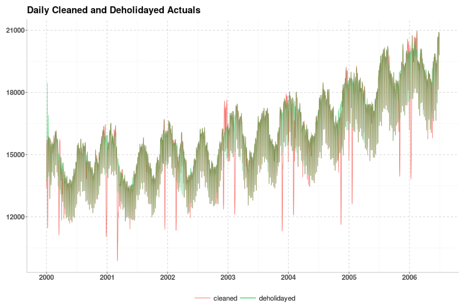
We forecast this time series from the middle of 2006 through the end of the data, for a 30-month forecast horizon. Our procedure first cleans the daily actuals as described above and then estimates holiday effects (based on a human-curated list). The two plots below show daily and weekly cleaned and de-holidayed values. After that, we conclude our forecast preparation by switching to weekly totals and accounting for seasonality effects (quantified at the bottom of this post).

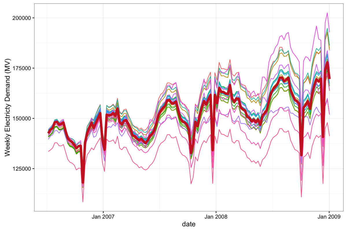
We then fit the models in our ensemble to the cleaned, de-holidayed, de-seasoned weekly time series. Once the individual models in our ensemble are fit to the time series, we can display the resulting forecasts from every model in the ensemble in the spaghetti-like plot below. The thicker, red line is the final forecast based on our selection and aggregation method while the other lines are the forecasts from individual models in the ensemble. The hope is that the diverse array of models will 'bracket the truth', in the sense described by Larrick and Soll (2006), leading to a better and more robust final forecast.
After converting our ensemble to a final forecast for each week of the forecast horizon, we re-season the data, distribute the weekly totals to the constituent days of the week for every week, and re-holiday the resulting daily values. From these we output final daily and weekly forecasts, as depicted below.
The plot below shows the entire time series and weekly forecasts for a 30-month forecast horizon starting in mid-2006.
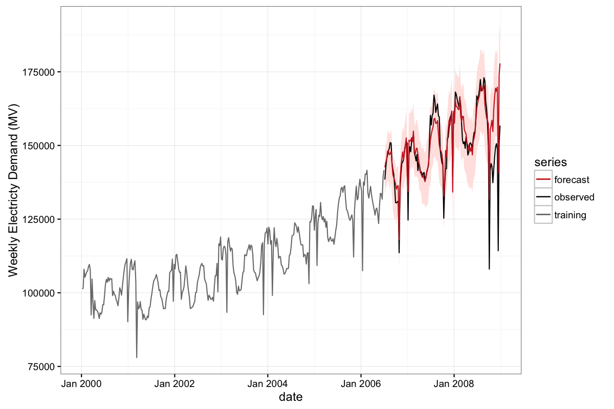
This next plot, also weekly, zooms in to focus on only the forecast period. This plot reveals reasonable forecast performance until about September 2008, ostensibly due to the impact in Turkey of the global Great Recession of 2008.

Now we show the daily forecast and observed data for a three-month period in mid-2008, covering a period 21 to 24 months into the forecast horizon.

Before the onset of the Great Recession’s impacts, the interquartile range of the percentage errors for the weekly forecast was 2.7%, from -1.2% to 1.5%. Corresponding numbers for the daily forecast were 3.2%, from -1.6% to 1.6%. The 10th and 90th percentiles were -3.5% and 2.8% for the weekly forecast, and -3.9% and 3.3% for the daily forecast. The median of the weekly percentage errors was 0.1% and was the same (0.1%) for the daily percentage errors. Absolute Percentage Errors told a similar story. Overall, the Mean Absolute Percentage Errors were 1.9% for the weekly forecast and 2.3% for the daily forecast.
Beyond the forecasts, our routine produces ancillary information with business relevance. For instance, immediately below we show the estimated holiday impacts for Eid al-Adha and Eid al-Fitr over a span of about 14 days surrounding the particular holiday (anchored about a 'zero' day on the horizontal axis.) Farther below, we show annual estimated seasonality (weekly resolution), past and forecast. Both estimated holiday impacts and seasonal adjustment factors are expressed on relative scales. While important to business understanding in their own right, it is worth saying one last time that doing a good job estimating seasonal and holiday effects reduces the burden on the models in the ensemble, helping them to better identify long-term growth trends.


[2] Cleveland, Robert B., William S. Cleveland, and Irma Terpenning. "STL: A seasonal-trend decomposition procedure based on loess." Journal of Official Statistics 6.1 (1990): 3.
[3] Clemen, Robert T. "Combining forecasts: A review and annotated bibliography." International journal of forecasting 5.4 (1989): 559-583
[4] Bates, John M., and Clive WJ Granger. "The combination of forecasts." Journal of the Operational Research Society 20.4 (1969): 451-468.
[5] Makridakis, Spyros, and Michele Hibon. "The M3-Competition: results, conclusions and implications." International journal of forecasting 16.4 (2000): 451-476.
[6] Mannes, Albert E., Jack B. Soll, and Richard P. Larrick. "The wisdom of select crowds." Journal of personality and social psychology 107.2 (2014): 276.
[7] Murray Stokely, Farzan Rohani, and Eric Tassone. “Large-Scale Parallel Statistical Forecasting Computations in R”, Google Research report.
[8] De Livera, Alysha M., Rob J. Hyndman, and Ralph D. Snyder. "Forecasting time series with complex seasonal patterns using exponential smoothing." Journal of the American Statistical Association 106.496 (2011): 1513-1527.
[9] Larrick, Richard P., and Jack B. Soll. "Intuitions about combining opinions: Misappreciation of the averaging principle." Management science 52.1 (2006): 111-127. APA
We were part of a team of data scientists in Search Infrastructure at Google that took on the task of developing robust and automatic large-scale time series forecasting for our organization. In this post, we recount how we approached the task, describing initial stakeholder needs, the business and engineering contexts in which the challenge arose, and theoretical and pragmatic choices we made to implement our solution.
Introduction
Time series forecasting enjoys a rich and luminous history, and today is an essential element of most any business operation. So it should come as no surprise that Google has compiled and forecast time series for a long time. For instance, the image below from the Google Visitors Center in Mountain View, California, shows hand-drawn time series of “Results Pages” (essentially search query volume) dating back nearly to the founding of the company on 04 September 1998.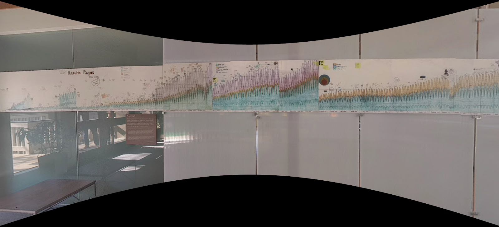 |
Hand-Drawn Time Series of Google “Results Pages”, November 1998 through July 2004. Due to multiple changes to the scale of the values depicted on the vertical axis, “Results Pages” values, which reflect search query volume, at the rightward end of the plot (corresponding to July 2004) are 2000 times larger than the values depicted at the leftward end (corresponding to November 1998).
The demand for time series forecasting at Google grew rapidly along with the company over its first decade. Various business and engineering needs led to a multitude of forecasting approaches, most reliant on direct analyst support. The volume and variety of the approaches, and in some cases their inconsistency, called out for an attempt to unify, automate, and extend forecasting methods, and to distribute the results via tools that could be deployed reliably across the company. That is, for an attempt to develop methods and tools that would facilitate accurate large-scale time series forecasting at Google.
Our team of data scientists and software engineers in Search Infrastructure was already engaged in a particular type of forecasting. For us, demand for forecasts emerged from a determination to better understand business growth and health, more efficiently conduct day-to-day operations, and optimize longer-term resource planning and allocation decisions. Because our team was already forecasting a large number of time series for which direct analyst implementation and supervision were impractical, it was well positioned to attempt such a unification, automation, and distribution of forecasting methods.
In the balance of this post, we will discuss and demonstrate aspects of our forecasting approach.
- We begin by describing our general framework for thinking about our task, which entails carefully defining the overall forecasting problem -- what it is and what it is not -- and decomposing the problem into tractable subproblems whenever possible.
- We then detail subproblems resulting from the decomposition, and our approaches to solving them.
- Adjustments to clean the data: missing values, anomalies, level changes, and transformations.
- Adjustments for effects: holiday, seasonality, and day-of-week effects.
- Disaggregation of the time series into subseries and reconciliation of the subseries forecasts.
- Selection and aggregation of forecasts from an ensemble of models to produce a final forecast.
- Quantification of forecast uncertainty via simulation-based prediction intervals.
GENERAL FRAMEWORK
A critical learning from our forecasting endeavor was the value of careful thought about the environment in which both the problem and potential solutions arise. The challenge, of course, is in the details: What problem are we trying to solve and -- just as importantly -- what problems are we not trying to solve? How do we carefully delineate and separate where possible the various subproblems that make up the problem we are trying to solve? Which subproblems should be decoupled and treated independently to better attack them or for ease of implementation?Our Forecasting Problem
Our typical use case was to produce a time series forecast at the daily level for a 12-24 month forecast horizon based on a daily history two or more years long. On occasion, we might be interested in forecasting based on weekly totals or a move to a more refined temporal resolution, such as hours or minutes, but the norm was daily totals. Other times we might be asked to make a forecast based on a shorter history.In terms of scope, we sought to forecast a large number of time series, and to do so frequently. We wanted to forecast a variety of quantities: overall search query volume and particular types of queries; revenue; views and minutes of video watched on Google-owned YouTube (which recently reached a billion hours daily); usage of sundry internal resources; and more. Additionally, we often had an independent interest in subseries of those quantities, such as disaggregated by locale (e.g., into >100 countries or regions), device type (e.g., by desktop, mobile, and tablet), and operating system, as well as combinations of all these (e.g., locale-by-device type.) Given the assortment of quantities and their combinatorial explosion into subseries, our forecasting task was easily on the order of tens of thousands of forecasts. And then we wanted to forecast these quantities every week, or in some cases more often.
The variety and frequency of forecasts demanded robust, automatic methods --- robust in the sense of dramatically reducing the chance of a poor forecast regardless of the particular characteristics of the time series being forecast (e.g., its growth profile) and automatic in the sense of not requiring human intervention before or after running the forecast.
Another important domain constraint was that our time series were the result of some aggregate human phenomenon --- search queries, YouTube videos viewed, or (as in our example) electricity consumed in Turkey. Unlike physical phenomena such as earthquakes or the tides, the time series we forecast are shaped by the rhythms of human civilization and its weekly, annual, and at-times irregular and evolving cycles. Calendaring was therefore an explicit feature of models within our framework, and we made considerable investment in maintaining detailed regional calendars.
Non-Problems
"Forecasting" is in many ways an overloaded word, with many potential meanings. We certainly were not trying to handle all forecasting possibilities, which sometimes vexed our colleagues who had turned to us for assistance. So what did "forecasting" not mean to us?Our initial use case did not involve explanatory variables, instead relying only the time series histories of the variables being forecast. Our rationale was in accord with the views expressed in the online forecasting book by Hyndman and Athanasopoulos [1], who after mentioning the potential utility of an "explanatory model" write:
However, there are several reasons a forecaster might select a time series model rather than an explanatory model. First, the system may not be understood, and even if it was understood it may be extremely difficult to measure the relationships that are assumed to govern its behavior. Second, it is necessary to know or forecast the various predictors in order to be able to forecast the variable of interest, and this may be too difficult. Third, the main concern may be only to predict what will happen, not to know why it happens. Finally, the time series model may give more accurate forecasts than an explanatory or mixed model.
"Forecasting" for us also did not mean using time series in a causal inference setting. There are tools for this use case, such as Google-supported CausalImpact.
CausalImpact is powered by bsts (“Bayesian Structural Time Series”), also from Google, which is a time series regression framework using dynamic linear models fit using Markov chain Monte Carlo techniques. The regression-based bsts framework can handle predictor variables, in contrast to our approach. Facebook in a recent blog post unveiled Prophet, which is also a regression-based forecasting tool. But like our approach, Prophet aims to be an automatic, robust forecasting tool.
At lastly, "forecasting" for us did not mean anomaly detection. Tools such as Twitter’s AnomalyDetection or RAD ("Robust Anomaly Detection") from Netflix, as their names suggest, target this type of problem.
Decomposing our problem
Our ultimate objective is to accurately forecast the expected growth trends of our time series. To do so, we have found it useful to make a variety of cleaning adjustments and effects adjustments to better isolate the underlying growth trend. Both cleaning and effects adjustments allow for better estimation of underlying trend. The difference is that cleaning is to remove unpredictable nuisance artifacts whereas the effects are regular patterns we wish to capture explicitly. Thus our forecasting routine decomposes our overall problem into subproblems along these very lines.Cleaning Adjustments
At the start of our process, we make several cleaning adjustments to the observed time series. Four major cleaning adjustments that we treat as separate problems are (a) missing values, (b) presumed anomalies, (c) accounting for abrupt level changes in the time series history, and (d) any transformations likely to result in improved forecast performance. Pre-processing our time series with these cleaning adjustments helps them to better conform to the assumptions of forecasting models to be fit later, such as stationarity.Missing values and putative anomalous values may present as a dramatic spike or drop not explained by a launch, seasonality effect, or holiday impact. They can arise from data collection errors or other unlikely-to-repeat causes such as an outage somewhere on the Internet. If unaccounted for, these data points can have an adverse impact on forecast accuracy by disrupting seasonality, holiday, or trend estimation.
Level changes are different in that they represent a more permanent change in the level of the time series, in contrast to anomalies, where the time series returns to its previous level at trend after a brief period. They may result from launches, logging changes, or external events. At a minimum, adjusting for level changes results in a longer effective time series, and often makes trend estimation easier when the models are finally fit.
We also permit transformations, such as a Box-Cox transformation. These can be automatic (the default setting for some models) or user-specified. These too can help with meeting model assumptions and with eventual forecast accuracy (final forecasts must be re-transformed to the original scale, of course).
Effect Adjustments
Typically we also adjust for several effects before fitting our models (an exception being seasonality in STL models which the models directly handled [2]). There are three major effects that we decouple and treat as subproblems: holiday effects, seasonality effects, and day-of-week effects. Whereas cleaning adjustments pre-process the data and are mostly targeted at one-off incidents, the other effects we attempt to adjust for are typically repeated patterns.For the effect adjustments we seek to: quantify the effect; remove the effect from the time series; forecast the time series without the effect; and re-apply the effect to that forecast post hoc. By contrast, for cleaning adjustments, we seek only to quantify, so as to remove. In addition, for the effect adjustments, we typically have business-knowledge or day-to-day-operations motivations for wanting to know the magnitude of the effect; this is not always the case for cleaning adjustments.
Though not cleanly separated conceptually, holiday effects and seasonality effects are partially distinguished in that seasonality effects are defined as occurring during the same numerical week of the year, whereas holiday effects are specific to the day of the occurrence and adjacent "shoulder" days. That said, some holidays fall on the same calendar day but on a different day of the week each year, such as Independence Day falling on the 4th of July in the United States; some fall on the same day of the week and week of the year, but on a different calendar day, such as Thanksgiving Day falling on the fourth Thursday of November in the United States; and some vary with solar or lunar phenomena, such as the Easter Sunday holiday celebrated in many countries around the world, which can fall anywhere from late March to late April. Due to these differences, some holiday effects and seasonality effects may not be identifiable. But note the use of "week" as the germane unit of time for seasonality and "day" for holidays: We estimate holiday effects from the adjusted daily data, but then roll up daily values to weekly totals before estimating seasonality effects.
Estimating holiday and seasonality effects is more art than science due to the paucity of relevant historical data. For instance, to estimate the effect of Independence Day when it falls on a weekday versus a weekend, you can accrue observations only so fast! And the effect may evolve as, say, smart phones proliferate and people begin doing more Google Maps searches the evening of Independence Day. Our experience with holiday adjustments is that ad hoc methods which work well and are easily interpretable (if only for debugging) are preferred to elegant, comprehensive mathematical models which may not deliver nor are amenable to a postmortem when something (inevitably) goes wrong.
The plots below illustrate a toy example of cleaning and effects adjustments in action. In the first plot, the raw weekly actuals (in red) are adjusted for a level change in September 2011 and an anomalous spike near October 2012. The cleaned weekly actuals (in green) are much smoother, but still show strong seasonal and holiday effects. As noted above, these are estimated, removed, the long-term trend is forecast, and then the seasonal and holiday effects are added back, producing the weekly forecast (in blue), as shown in the second plot.
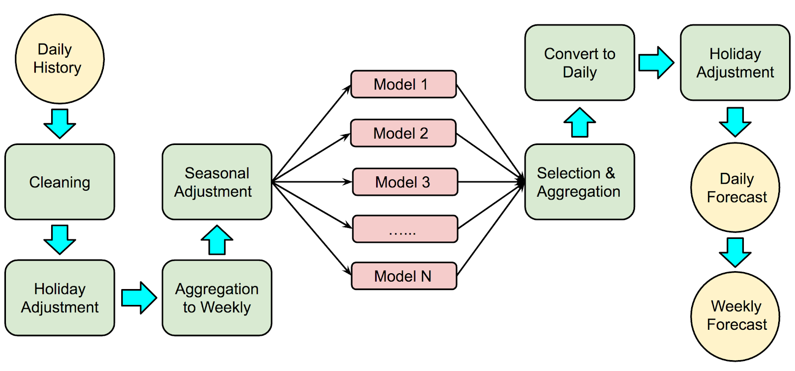
The block diagram below shows where these cleaning and effects adjustments occur in the overall sequence of our forecast procedure:
Day-of-Week Effects
By "day-of-week effects" we mean a contributor to the multiple seasonalities of daily data typically observed --- there is often one pattern with period seven and then one or more patterns with much larger periods corresponding to an annual cycle. There are often multiple calendars operating within any geography (to name just two possible calendars, Islamic and Gregorian calendars have different periods and often produce more than one annual cycle in certain locales). Again, we decompose our overall problem and treat this day-of-week effect as its own problem, on its own terms. That is, after the cleaning adjustments and after de-holidaying and de-seasoning the data, our initial output is a weekly forecast from rolled-up weekly totals. Thus for daily forecasts we are left with distributing weekly totals to daily values.In our experience there are great dividends in treating the forecasting task, with its priority on growth trend estimation, separately from the day-of-week effect. By decomposing the overall problem, we can focus on methods that best solve the specific subproblem. For us, forecasting the trend from less noisy weekly data (again, and importantly, after cleaning and effect adjustments) results in better growth trend estimation compared to all-in-one methods. Methods that attempt to simultaneously estimate all relevant parameters in a unified framework may be vulnerable to omission, overfitting, confounding of effects, or something else going awry which subsequently impairs the method's ability to accurately estimate the growth trend.
Likewise, by treating the day-of-week effect on its own we can deploy methods targeted to capturing its important aspects. For instance, in our data we often see secular trends as well as annual seasonality in the amplitude of the weekly cycle i.e., long-term changes to the proportions of the weekly total going to each day of the week and intra-year cycles in these proportions. A model general enough to accommodate such phenomena, and everything else, along with the data to identify all relevant parameters is for us too much to ask. Such a model risks conflating important aspects, notably the growth trend, with other less critical aspects.
Disaggregation And Reconciliation
Apart from the cleaning and effect adjustments, we may decompose our overall problem for other reasons. Earlier we mentioned that we often had an independent interest in subseries of a parent time series, such as disaggregated by locale, device type, operating system, and combinations of these. Yet even when we do not have an independent interest in the subseries, forecasting the constituent parts (and indeed the entire hierarchy that results from this type of disaggregation) and then reconciling all those forecasts in some manner to produce a final forecast of the parent time series is typically more accurate and robust than only forecasting the parent time series itself directly. This type of decomposition is quite literal --- we turn the task of forecasting one time series into that of forecasting many subseries and then reconciling them.Consider, for example, Global search queries. The first step, disaggregation, is quite natural. Search queries are logged with many attributes, and we typically use at least geography and device type. This aspect is easy. Next, forecasting the many subseries: Again, this is easy --- our forecast methodology is designed to be robust and automatic, so dramatically increasing the number of forecasts is not overly risky, either. Lastly, however, we need a method to take this collection of forecasts and reconcile them. This is more challenging.
A simple solution is to forecast only at the bottom of the hierarchy and simply sum the forecasts to produce an overall parent forecast (and indeed forecasts all throughout the hierarchy.) This can be quite effective, as the important differences in growth profiles tend to arise across the geography-by-device-type boundaries, and forecasting them independently as a first step frees them.
An obvious requisite property of reconciliation is arithmetic coherence across the hierarchy (which is implicit in the sum-up-from-the-bottom possibility in the previous paragraph), but more sophisticated reconciliation may induce statistical stability of the constituent forecasts and improve forecast accuracy across the hierarchy. While we use reconciliation methods tailored to our specific context, similar techniques have been implemented in the R package hts and written about in the literature.
Ensemble Methods
In keeping with our goals of robustness and automation, we turned to ensemble methods to forecast growth trends. In a time series context, ensemble methods generally fit multiple forecast models and derive a final forecast from the ensemble, perhaps via a weighted average, in an attempt to produce better forecast accuracy than might result from any individual model.Though more sophisticated, more mathematically alluring options are available for producing a final forecast from an ensemble, such as Bayesian Model Averaging, we opt for simple approaches. The confluence of our beliefs about the world, underlying theoretical results, and empirical performance compel us toward deriving a final forecast from the ensemble via a simple measure of central tendency (i.e., a mean or median) after some effort to remove outliers (which could be as simple as trimming or winsorizing.) Crucially, our approach does not rely on model performance on holdout samples. Details follow, but first an exploration of why such an embarrassingly simple and seemingly ad hoc approach might do so well in this setting.
Why do simple methods perform well?
When it comes to obtaining a final forecast from an ensemble, the following quote from Clemen [3] gives us the lay of a land not entirely welcoming to the mathematical statistician (emphasis added):In many studies, the average of the individual forecasts has performed best or almost best. Statisticians interested in modeling forecasting systems may find this state of affairs frustrating. The questions that need to be answered are (1) why does the simple average work so well, and (2) under what conditions do other specific methods work better?
Clemen then homes in on a contradiction inherent in the pursuit of sophisticated combination strategies (emphasis added):
From a conventional forecasting point of view, using a combination of forecasts amounts to an admission that the forecaster is unable to build a properly specified model. Trying ever more elaborate combining models seems only to add insult of injury, as the more complicated combinations do not generally perform all that well.
With that context, consider an example inspired by Bates and Granger [4] and by [3]. Define two independent random variables $X_1 \sim N(0, 1)$ and $X_2 \sim N(0, 2)$. For this simple vignette, we might regard $X_1$ and $X_2$ as errors from a measuring scale and note that $X_2$ is not as precise an instrument as $X_1$. Define
$$
X_A = \frac{1}{2} X_1 + \frac{1}{2} X_2
$$From basic theory, $X_A \sim ~ N(0, \frac{3}{4})$. In other words, the simple, unweighted average of these particular $X_1$ and $X_2$ has smaller variance than $X_1$ even though we combined $X_1$ in equal measure with a less precise instrument, $X_2$. Now, if the variances of $X_1$ and $X_2$ were truly known to be $1$ and $2$, respectively, [4] would suggest we form $$
X_C = k X_1 + (1 - k) X_2
$$with $k = 2/3$ to minimize the variance of $X_C$. Thus $X_C \sim N(0, \frac{2}{3})$, which would be a superior instrument compared to $X_A$ with its variance of $\frac{3}{4}$.
However, consider another scenario. Suppose $X_1$ and $X_2$ are independent as before, but now suppose we only know that one of $X_1$ and $X_2$ is distributed as $N(0, 1)$ and the other as $N(0, 2)$, and we do not know which is which. Thus with equal chance we might have $X_1 \sim N(0, 1)$ and $X_2 \sim N(0, 2)$ or $X_1 \sim N(0, 2)$ and $X_2 \sim N(0, 1)$. Let’s again form $X_A$ and $X_C$ as before. $X_A$ is unchanged, regardless of how $X_1$ and $X_2$ are actually distributed, with $X_A \sim N(0, \frac{3}{4})$. If $X_1$ has the lower variance we once again have $X_C \sim N(0, \frac{2}{3})$. But if it is the case that $X_1 \sim N(0, 2)$ and $X_2 \sim N(0, 1)$, then the variance of $X_C$ would be $1$. This would be an inferior instrument compared to $X_A$ with its variance of $\frac{3}{4}$.
Overall, when the weights are placed correctly $X_C$ is a slightly better instrument compared to $X_A$, but when the weights are placed incorrectly, $X_C$ is substantially inferior to $X_A$. In other words, there is an asymmetry of risk-reward when there exists the possibility of misspecifying the weights in $X_C$. Consequently, our confidence in departing from a simple, unweighted average of models in favor of preferential weighting should be shaped by how much we believe (or can demonstrate) that we can know the future precision of the instruments we deploy, as well as our risk tolerance.
In our forecasting routine, we face a similar conundrum: Do we believe (or can we demonstrate) that the performance of the models in the ensemble on what is often a short holdout period is sufficiently predictive of relative future forecast accuracy of the ensemble’s models to warrant a departure from a simple average based on equal weights? Relatedly, what do we believe about the process that generates the data we see?
In our view, the data we observe are not from a deterministic casino game with known probabilities or from physical laws embedded in the fabric of the Universe. Our data arise from a complex, human process; our data depend on "fads and fashions"; our data are infused with all the psychology and contradiction that is human existence; our data will eventually reflect -- and more likely, soon reflect! -- unknowable unknowns, future ideas and inventions yet to be developed, novel passions and preferences; in short, our data are far from stationary. It is worth quoting Makridakis and Hibon [5] extensively here, for we share their view:
The reason for the anomalies between the theory and practice of forecasting is that real-life time series are not stationary while many of them also contain structural changes as fads, and fashions can change established patterns and affect existing relationships. Moreover, the randomness in such series is high as competitive actions and reactions cannot be accurately predicted and as unforeseen events (e.g., extreme weather conditions) affecting the series involved can and do occur. Finally, many time series are influenced by strong cycles of varying duration and lengths whose turning points cannot be predicted, making them behave like a random walk.
When the context in which the data arises changes, even a well-executed cross validation provides inadequate protection against overfitting. Instead of overfitting to the observed data in the usual sense, the risk is in overfitting to a context that has changed. In our view, this is fundamentally what makes our forecasting problem different from other prediction problems.
For such reasons, we place strong prior belief on simple methods to convert the ensemble into a final forecast. The decision not to rely on performance in a holdout sample was no mere implementation convenience. Rather, it best reflects our beliefs about the state of the world -- “that real-life time series are not stationary” -- while also best conforming to our overarching goal of an automatic, robust forecasting routine that minimizes the chance of any catastrophically bad forecast.
What’s in our ensemble?
So, what models do we include in our ensemble? Pretty much any reasonable model we can get our hands on! Specific models include variants on many well-known approaches, such as the Bass Diffusion Model, the Theta Model, Logistic models, bsts, STL, Holt-Winters and other Exponential Smoothing models, Seasonal and other other ARIMA-based models, Year-over-Year growth models, custom models, and more. Indeed, model diversity is a specific objective in creating our ensemble as it is essential to the success of model averaging. Our aspiration is that the models will produce something akin to a representative and not overly repetitive covering of the space of reasonable models. Further, by using well-known, well-vetted models, we attempt to create not merely a "wisdom of crowds" but a "wisdom of crowds of experts" scenario, in the spirit of Mannes [6].As an implementation detail, though, we provide flags in our code so that an analyst could abandon the default settings and force any particular model to be in or out of the ensemble. This imbues the forecasting routine with two attractive properties. First, an analyst who wishes to add a new model to the ensemble can do so with little risk of degrading the performance of the ensemble as a whole. In fact, the expectation is that a good-faith addition of a new model will do no harm and may improve the overall performance of a final forecast from the ensemble. Such future-proofing is a virtue. Second, if an analyst is insistent on running only their own new model it will now sit in the middle of the entire production pipeline that will handle all the adjustments previously discussed. In other words, their new model will not be at a disadvantage in terms of the adjustments.
Selection and aggregation: from ensemble to final forecast
For each week of the forecast horizon, we convert the models into a final forecast for that week. Though more sophisticated possibilities exist, in our initial approach we treat the collection of forecasts in the ensemble for a given week independently of other weeks. We then compute a simple trimmed mean of all the models passing some basic sanity checks. Since there is always the risk of an absurd forecast (e.g., going to zero or zooming off toward infinity) from any member of the ensemble, due to numerical problems or something else, we recommend an approach with some form of outlier removal. With such an approach, it is not uncommon for the final forecast to achieve predictive accuracy superior to any individual model. Over the many time series we forecast it is typically at or near the top -- delivering the type of robustness we desire.Prediction Intervals
A statistical forecasting system should not lack uncertainty quantification. In addition, there is often interest in probabilistic estimates of tail events, i.e., how high could the forecast reasonably go? In our setup some of our previous choices, notably ensembling, break any notion of a closed-form prediction interval. Instead, we use simulation-based methods to produce prediction intervals.Our approach (illustrated below) uses historical k-week-out errors to drive the simulations. In a simple case the one-week-out errors suffice, and the simulation proceeds iteratively: forecast one week forward, perturb this forecast with a draw from the error distribution, and repeat 52 times for a one-year realization; then do this, say, $1000$ or $10,000$ times and take quantiles of the realizations as uncertainty estimates. The process is inherently parallel: Each realization can be produced independently by a different worker machine. Empirical coverage checks are recommended, of course, as is assessment of any autocorrelation in the k-week-out errors.
 |
| Simulating prediction errors |
While producing prediction intervals is computationally intensive, the Google environment features abundant, fast parallel computing. This shaped the evolution of our approach, making possible and selecting out as advantageous such a computationally intensive technique. Please see [7] for additional details.
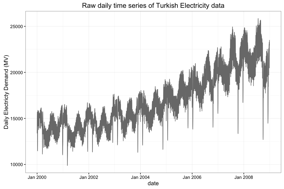
Example: Turkish Electricity data
To better illuminate our forecasting routine, we provide an example based on Turkish electricity data presented in De Livera [8] and available as a .csv file here. Below are daily and weekly totals of electricity demand (in MV) in Turkey from the start of 2000 through the end of 2008. As noted by [8], these data exhibit complex, multiple, and non-nested seasonal patterns owing to two annual seasonalities induced by the Islamic and Gregorian calendars as well as a weekly cycle that differs during the year. There is also apparent long-term trend and holiday impacts, and in principle these and the aforementioned seasonal patterns could be changing over time.We forecast this time series from the middle of 2006 through the end of the data, for a 30-month forecast horizon. Our procedure first cleans the daily actuals as described above and then estimates holiday effects (based on a human-curated list). The two plots below show daily and weekly cleaned and de-holidayed values. After that, we conclude our forecast preparation by switching to weekly totals and accounting for seasonality effects (quantified at the bottom of this post).
We then fit the models in our ensemble to the cleaned, de-holidayed, de-seasoned weekly time series. Once the individual models in our ensemble are fit to the time series, we can display the resulting forecasts from every model in the ensemble in the spaghetti-like plot below. The thicker, red line is the final forecast based on our selection and aggregation method while the other lines are the forecasts from individual models in the ensemble. The hope is that the diverse array of models will 'bracket the truth', in the sense described by Larrick and Soll (2006), leading to a better and more robust final forecast.
After converting our ensemble to a final forecast for each week of the forecast horizon, we re-season the data, distribute the weekly totals to the constituent days of the week for every week, and re-holiday the resulting daily values. From these we output final daily and weekly forecasts, as depicted below.
The plot below shows the entire time series and weekly forecasts for a 30-month forecast horizon starting in mid-2006.
This next plot, also weekly, zooms in to focus on only the forecast period. This plot reveals reasonable forecast performance until about September 2008, ostensibly due to the impact in Turkey of the global Great Recession of 2008.
Now we show the daily forecast and observed data for a three-month period in mid-2008, covering a period 21 to 24 months into the forecast horizon.
Before the onset of the Great Recession’s impacts, the interquartile range of the percentage errors for the weekly forecast was 2.7%, from -1.2% to 1.5%. Corresponding numbers for the daily forecast were 3.2%, from -1.6% to 1.6%. The 10th and 90th percentiles were -3.5% and 2.8% for the weekly forecast, and -3.9% and 3.3% for the daily forecast. The median of the weekly percentage errors was 0.1% and was the same (0.1%) for the daily percentage errors. Absolute Percentage Errors told a similar story. Overall, the Mean Absolute Percentage Errors were 1.9% for the weekly forecast and 2.3% for the daily forecast.
Beyond the forecasts, our routine produces ancillary information with business relevance. For instance, immediately below we show the estimated holiday impacts for Eid al-Adha and Eid al-Fitr over a span of about 14 days surrounding the particular holiday (anchored about a 'zero' day on the horizontal axis.) Farther below, we show annual estimated seasonality (weekly resolution), past and forecast. Both estimated holiday impacts and seasonal adjustment factors are expressed on relative scales. While important to business understanding in their own right, it is worth saying one last time that doing a good job estimating seasonal and holiday effects reduces the burden on the models in the ensemble, helping them to better identify long-term growth trends.
Conclusion
To summarize, key to our own attempt at a robust, automatic forecasting methodology was to divide and (hopefully) conquer where possible as well as to implement ensemble methods in accord with our risk tolerance and our beliefs about the data generating mechanism. But as anyone involved real-world forecasting knows, this is a complex space. We are eager to hear from practicing data scientists about their forecasting challenges --- how they might be similar to or differ from our problem. We hope this blog post is the start of such a dialogue.
References
[1] Hyndman, Rob J., and George Athanasopoulos. Forecasting: principles and practice. OTexts, 2014. http://otexts.org/fpp/. Accessed on 20 March 2017. Specifically, see "1.4 Forecasting data and methods".[2] Cleveland, Robert B., William S. Cleveland, and Irma Terpenning. "STL: A seasonal-trend decomposition procedure based on loess." Journal of Official Statistics 6.1 (1990): 3.
[3] Clemen, Robert T. "Combining forecasts: A review and annotated bibliography." International journal of forecasting 5.4 (1989): 559-583
[4] Bates, John M., and Clive WJ Granger. "The combination of forecasts." Journal of the Operational Research Society 20.4 (1969): 451-468.
[5] Makridakis, Spyros, and Michele Hibon. "The M3-Competition: results, conclusions and implications." International journal of forecasting 16.4 (2000): 451-476.
[6] Mannes, Albert E., Jack B. Soll, and Richard P. Larrick. "The wisdom of select crowds." Journal of personality and social psychology 107.2 (2014): 276.
[7] Murray Stokely, Farzan Rohani, and Eric Tassone. “Large-Scale Parallel Statistical Forecasting Computations in R”, Google Research report.
[8] De Livera, Alysha M., Rob J. Hyndman, and Ralph D. Snyder. "Forecasting time series with complex seasonal patterns using exponential smoothing." Journal of the American Statistical Association 106.496 (2011): 1513-1527.
[9] Larrick, Richard P., and Jack B. Soll. "Intuitions about combining opinions: Misappreciation of the averaging principle." Management science 52.1 (2006): 111-127. APA
Hi, great post.
ReplyDeleteAs a note would be interesting to see some results metrics from individual forecasting methods vs the ensamble one.
Cheers,
Hi!
DeleteThank you for your comment. While we could show such results for this one example time series (in which the final model derived from the ensemble performed consistently among the top handful of models over the forecast horizon, if memory serves), we believe the issue you raise is even more interesting and more in accord with the forecasting challenge we faced if considered over a large number of time series (100s or 1000s). We hope to post an update or perhaps a new blog post showing this type of performance, i.e., over a large number of time series, some time soon.
Cheers,
Eric
Hello, Thanks for the great write-up. It would be great if at least part of this work made it to the open-source community!
ReplyDeleteHi Alek,
DeleteThank you for your comment and suggestion. If there is any update on this, we will reply again to this comment.
Cheers,
Eric
That is a heck of a lot of time to hand draw time series. I always love to see ggplot graphs in articles.
ReplyDeleteHi Matt,
DeleteYes, aren't the hand-drawn time series impressive? Thank you for your comments!
Cheers,
Eric
Hi,
ReplyDeleteCan you please provide some insight into how to get the fitted values in the bsts method? Thanks.
Hi Ojaswini,
DeleteThank you for your comment. Please check out the links below, which may shed light on your question. For link [3], please note that bsts offers a predict method (predict.bsts). Also, please stay tuned to this space, as bsts may be the subject of a future blog post.
Cheers,
Eric
[1] https://sites.google.com/site/stevethebayesian/googlepageforstevenlscott/course-and-seminar-materials/bsts-bayesian-structural-time-series
[2] http://people.ischool.berkeley.edu/~hal/Papers/2013/pred-present-with-bsts.pdf
[3] https://cran.r-project.org/web/packages/bsts/index.html
I believe the approach is outstanding, especially the way the team rationalized using an ensemble of methods, dis-aggregating, and re-conciliating to obtain forecasts. The application of seasonal effects to characterize trends in weeks, years, and holidays was eye-opening. One thing I would like to see in the model is the inclusion of an explanatory model with explanatory variables (perhaps as part of the ensemble). The Turkish Electricity data seems reasonably unaffected by any global or local events until the recession in 2008, but I would not believe that the impacts of global and local events will not be outliers in the near future or present, given how interdependent the world is becoming. with forecasts. The average was taken from the ensemble, but do you think it would improve results to take a weighted average of the ensemble based on the accuracy of the technique? These weights could also be seasonal.
ReplyDeleteHi,
DeleteThank you for your comment.
In principle there is nothing forbidding the use of models with explanatory variable in the ensemble. The passage where we quoted Rob Hyndman describes some practical challenges to doing so, but there may be cases where this will be beneficial and not unduly burdensome.
As for your other point, and to misquote Tom Petty and the Heartbreakers, the weighting is the hardest part [ https://youtu.be/uMyCa35_mOg ] -- at least for us in the context in which our forecasting challenge arises. There may be contexts where weighting results in improved forecast performance, to be sure. This could happen the way you suggest (seasonal), or it could be that time series with certain characteristics are better forecast by certain types of models, or it could be that different models do a better job at different points in the forecast horizon, or something else. However, for our forecasting challenge, given the number and diversity of time series we faced, our risk-reward preferences, and our beliefs about the way our data arose, we preferred the approach described in the blog post.
Cheers,
Eric
Hi,
ReplyDeleteCould you elaborate a little more in the code or methods used for cleaning?.
Thank you!
Hi Jose,
DeleteThank you for your comment. As with a previous comment, this too could form the basis of a substantial update to this post or provide the basis of a new blog post. We will update here if and when either of those are in the works.
Cheers,
Eric
Was reading through this recent google data science blog on forecasting time series, and they have a pretty extended discussion as to why they favor aggregating forecasts via the median or average as opposed to more sophisticated techniques (using cross validation to pick the weights, bayesian model averaging etc). They make some good points about non-stationarity / non-realizability as to why cross validation doesn't work, and they present a toy example where an ensemble predictor can do much worse
ReplyDeletethan a single predictor if the aggregation weights are slightly off. What I don't get about this article is why wouldn't you use exponential weights to aggregate forecasts? Then the toy example falls apart because at least asymptotically you have vanishing regret O(log(k)/n^1.2) I believe to the optimal forecaster. Maybe I'm missing something obvious?
Lovely post, I especially liked how you've introduced the framework and I agree explanatory variables very seldom help. I've personally used ensemble models with decent success on similar short-term and long-term horizons.
ReplyDeleteHowever, I'd love to know your thoughts about using RNNs/LSTMs for time series forecasting since they're good at capturing long-term dependencies. Given the popularity of TensorFlow at Google, did your team try to use LSTMs for building models? What has been your experience? Do you think its possible to include them in such ensembles?
Awesome post. I've dealt with a lot of these issues in my line of work as well. For setting out-of-sample forecast accuracy expectations, have you tried using a form of k-fold cross validation where h is your forecast horizon, you take h-size test sets starting with your most recent data working backwards until you reach a minimum training set for model estimation?
ReplyDeleteIn regards to combining the ensemble members, you could also take the approach of the opera package and update the weighting of each ensemble member over time instead of using a robust central tendency measure.
If this is robust and automatic, how is it determined if a model is reasonable enough to be included in the ensemble without human intervention? I've found this to be vitally important, though obviously less important the higher the ensemble population gets.
Lastly, do you ever do any residual diagnostics of the ensemble? Could be interesting to ensure there aren't autocorrelations you're not taking into account.
Thanks for sharing this approach to forecasting. I frequently work with daily time series and after reading this post tried removing day of week effects, aggregating to weekly data and forecasting weekly using the bsts package. All that worked well but I can't figure out how to dis-aggregate the weekly daily and re-seasonalize it. Any help appreciated.
ReplyDeleteHas anyone used BSTS package, setting the parameters to mimic Prophet method? I think BSTS supports everything with the possible exception of change points in the trend estimation.
ReplyDelete