LSOS experiments: how I learned to stop worrying and love the variability
by AMIR NAJMI
In the previous post we looked at how large scale online services (LSOS) must contend with the high coefficient of variation (CV) of the observations of particular interest to them. In this post we explore why some standard statistical techniques to reduce variance are often ineffective in this “data-rich, information-poor” realm.
Despite a very large number of experimental units, the experiments conducted by LSOS cannot presume statistical significance of all effects they deem practically significant. We previously went into some detail as to why observations in an LSOS have particularly high coefficient of variation (CV). The result is that experimenters can’t afford to be sloppy about quantifying uncertainty. Estimating confidence intervals with precision and at scale was one of the early wins for statisticians at Google. It has remained an important area of investment for us over the years.
Given the role played by the variability of the underlying observations, the first instinct of any statistician would be to apply statistical techniques to reduce variability. “We have just emerged from a terrible recession called New Year's Day where there were very few market transactions,” joked Hal Varian, Google’s Chief Economist, recently. He was making the point that economists are used to separating the predictable effects of seasonality from the actual signals they’re interested in. Doing so makes it easier to study the effects of an intervention, say, a new marketing campaign, on the sales of a product. When analyzing experiments, statisticians can do something similar to go beyond overall comparisons between treatment and control. In this post we discuss a few approaches to removing the effects of known or predictable variation. These typically result in smaller estimation uncertainty and tighter interval estimates. Surprisingly, however, removing predictable variation isn’t always effective in an LSOS world where observations can have a high CV.
Variance reduction through conditioning
Suppose, as an LSOS experimenter, you find that your key metric varies a lot by country and time of day. There are pretty clear structural reasons for why this could be the case. For instance, the product offering of a personal finance website might be very different in different countries and hence conversion rates (acceptances per offer) might differ considerably by country. Or perhaps the kinds of music requested from an online music service vary a lot with hour of day, in which case the average number of songs downloaded per user session might vary greatly too. Thus any randomized experiment will observe variation in metric difference between treatment and control groups due merely to sampling variation in the number of experimental units in each of these segments of traffic. In statistics, such segments are often called “blocks” or “strata”. At Google, we tend to refer to them as slices.
One approach statisticians use to mitigate between-slices variability is to employ stratified sampling when assigning units to the treatment and the control group. Stratified sampling means drawing a completely randomized sample from within each slice, ensuring greater overall balance. Figure 1 illustrates how this would work in two dimensions.
 |
| Figure 1: Completely randomized versus stratified randomized sampling. |
To illustrate how this works, let’s take the music service as our example. Let the outcome variable $Y_i$ represent the number of songs downloaded in a user session $i$, assuming each user session is independent. To simplify the analysis, let’s further assume that the treatment does not affect the variance of $Y_i$. The simplest estimator for the average treatment effect (ATE) is given by the difference of sample averages for treatment and control:
\[
\mathcal{E}_1=\frac{1}{|T|}\sum_{i \in T}Y_i - \frac{1}{|C|}\sum_{i \in C}Y_i
\]
\mathcal{E}_1=\frac{1}{|T|}\sum_{i \in T}Y_i - \frac{1}{|C|}\sum_{i \in C}Y_i
\]
Here, $T$ and $C$ represent sets of indices of user sessions in treatment and control and $| \cdot |$ denotes the size of a set. The variance of this estimator is
\[
\mathrm{var\ } \mathcal{E}_1 = \left(\frac{1}{|T|} + \frac{1}{|C|} \right )\mathrm{var\ }Y
\]
Estimator $\mathcal{E}_1$ accounts for the fact that the number of treatment and control units may vary each time we run the experiment. However, it doesn't take into account the variation in the fraction of treatment and control units assigned to each hour of day. Conditioned on $|T|$ and $|C|$, the number of units assigned to treatment or control in each hour of day will vary according to a multinomial distribution. And since the metric average is different in each hour of day, this is a source of variation in measuring the experimental effect.
We can easily quantify this effect for the case when there is a constant experimental effect and variance in each slice. In other words, assume that in Slice $k$, $Y_i \sim N(\mu_k,\sigma^2)$ under control and $Y_i \sim N(\mu_k+\delta,\sigma^2)$ under treatment. To compute $\mathrm{var\ }Y$ we condition on slices using the law of total variance which says that \[
\mathrm{var\ }Y = E_Z[\mathrm{var\ }Y|Z] + \mathrm{var_Z}[EY|Z]
\]Let $Z$ be the random variable representing hour of day for the user session. $Z$ is our slicing variable, and takes on integer values $0$ through $23$. The first component, $E_Z[\mathrm{var\ }Y|Z]$, is the expected within-slice variance, in this case $\sigma^2$. The second component, $\mathrm{var_Z}[EY|Z]$, is the variance of the per-slice means. It's that part of the variance which is due to the slices having different means. We’ll call it $\tau^2$:
\begin{align}
\tau^2 &= \mathrm{var}_Z[EY|Z] \\
&= E_Z[(EY|Z)^2] - (E_Z[EY|Z])^2 \\
&= \sum_k w_k \mu_k^2 - \left( \sum_k w_k\mu_k \right )^2
\end{align}
where $w_k$ is the fraction of units in Slice $k$. In this situation, the variance of estimator $\mathcal{E}_1$ is
\tau^2 &= \mathrm{var}_Z[EY|Z] \\
&= E_Z[(EY|Z)^2] - (E_Z[EY|Z])^2 \\
&= \sum_k w_k \mu_k^2 - \left( \sum_k w_k\mu_k \right )^2
\end{align}
where $w_k$ is the fraction of units in Slice $k$. In this situation, the variance of estimator $\mathcal{E}_1$ is
\[
\mathrm{var\ } \mathcal{E}_1 = \left(\frac{1}{|T|} + \frac{1}{|C|} \right )(\sigma^2+\tau^2)
\]
Quantity $\tau^2$ is nonzero because the slices have different means. We can remove its effect if we employ an estimator $\mathcal{E}_2$ that takes into account the fact that the data are sliced:
\mathrm{var\ } \mathcal{E}_1 = \left(\frac{1}{|T|} + \frac{1}{|C|} \right )(\sigma^2+\tau^2)
\]
Quantity $\tau^2$ is nonzero because the slices have different means. We can remove its effect if we employ an estimator $\mathcal{E}_2$ that takes into account the fact that the data are sliced:
\[
\mathcal{E}_2=\sum_k \frac{|T_k|+|C_k|}{|T|+ |C|}\left( \frac{1}{|T_k|}\sum_{i \in T_k}Y_i - \frac{1}{|C_k|}\sum_{i \in C_k}Y_i \right)
\]
Here, $T_k$ and $C_k$ are the subsets of treatment and control indices in Slice $k$. This estimator improves on $\mathcal{E}_1$ by combining the per-slice average difference between treatment and control. Both estimators are unbiased. But the latter estimator has less variance. To see this, we can compute its variance:
\[
\mathrm{var\ } \mathcal{E}_2 =
\sum_k \left(\frac{|T_k|+|C_k|}{|T|+ |C|} \right )^2\left( \frac{1}{|T_k|} + \frac{1}{|C_k|} \right) \sigma^2
\]
Given that $|T_k| \approx w_k |T|$ and $|C_k| \approx w_k|C|$,
\begin{align}
\mathrm{var\ } \mathcal{E}_2 &\approx
\sum_k w_k^2 \left(\frac{1}{w_k|T|} + \frac{1}{w_k|C|} \right ) \sigma^2 \\
&=
\left(\frac{1}{|T|} + \frac{1}{|C|} \right ) \sigma^2
\end{align}
Intuitively, we have increased the precision of our estimator by using information in $Z$ about which treatment units happened to be in each slice and likewise for control. In other words, this estimator is conditioned on the sums and counts (sufficient statistics) in each slice rather than just overall sums and counts.
In general, we can expect conditioning to remove only effects due to the second component of the law of total variation. This is because $\mathrm{var}_Z [EY|Z]$ is the part of $\mathrm{var\ }Y$ explained by $Z$ while $E_Z[\mathrm{var\ }Y|Z]$ is the variance remaining even after we know $Z$. Thus, if an estimator is based on the average value of $Y$, we can bring its variance down to the fraction
\[
\frac{E_Z[\mathrm{var\ }Y|Z]}{\mathrm{var\ }Y}
\]
But that’s just the theory. As discussed in the last post, LSOS often face the situation that $Y$ has a large CV. But if the CV of $Y$ is large, it is often because the variance within each slice is large, i.e. $E_Z[\mathrm{var\ }Y|Z]$ is large. If we track a single metric across the slices, we do so because we believe more or less the same phenomenon is at work in each slice of the data. Obviously, this doesn’t have to be true. For example, an online music service may care about the fraction of songs listened to from playlists in each user session but this playlist feature may only be available to premium users. In this case, conditioning on user type could make a big difference to the variability. But then you have to wonder why the music service doesn’t just track this metric for premium user sessions as opposed to all user sessions!
Another way to think about this is that the purpose of stratification is to use side information to group observations which are more similar within strata than between strata. We have ways to remove the variability due to differences between strata (between-stratum variance). But if between-stratum variance is small compared to within-stratum variance, then conditioning is not going to be very effective.
Rare binary event example
In the previous post, we discussed how rare binary events can be fundamental to the LSOS business model. To that end, it is worth studying them in more detail. Let’s make this concrete with actual values. Say we have track the metric fraction of user sessions which result in a purchase. We care about the effect of experiments on this important metric.
Let $Y$ be the Bernoulli random variable representing the purchase event in a user session. Suppose that the purchase probability varies by hour of day $Z$. In particular, say $E[Y|Z]=\theta$ follows a sinusoidal function of hour of day varying by a factor of 3. In other words, $\theta$ varies from $\theta_{min}$ to $\theta_{max}=3 \theta_{min}$ with average $\bar{\theta} = (\theta_{min} + \theta_{max})/2$. In the plot below, $\theta_{min}=1\%$ and $\theta_{max}=3\%$.
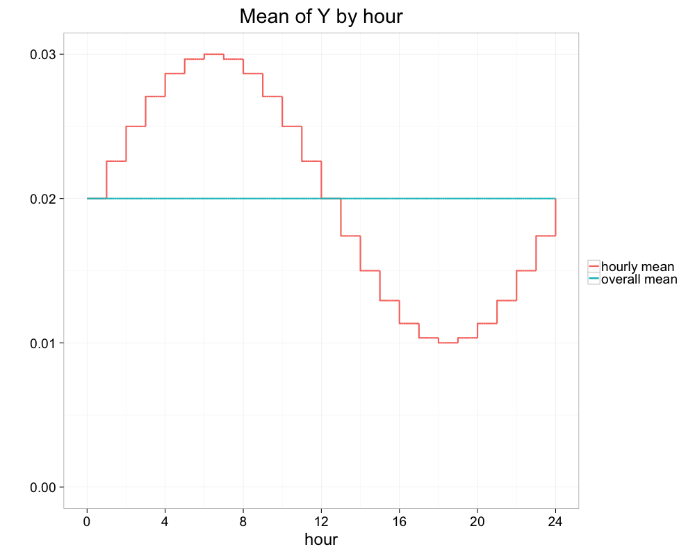 |
| Figure 2: Fictitious hourly variation in mean rate of sessions with purchase. |
For simplicity, assume there is no variation in frequency of user sessions in each hour of day. A variation in the hourly rate by a factor of 3 would seem worth addressing through conditioning. But we shall see that the improvement is small.
\[
\mathrm{var\ }Y = \bar{\theta}(1-\bar{\theta}) \\
\mathrm{var_Z}[EY|Z] = \mathrm{var\ }\theta
\]
We can approximate $\mathrm{var\ }\theta$ by the variance of a sine wave of amplitude $(\theta_{max} - \theta_{min})/2$. This gives us $\mathrm{var\ }\theta \approx (\theta_{max} - \theta_{min})^2/8$ which reduces to $\bar{\theta}^2/8$ when $\theta_{max}=3 \theta_{min}$. Thus the fraction of reducible variance is
\[
\frac{\mathrm{var\ }\theta}{\mathrm{var\ }Y} = \frac{\bar{\theta}}{8(1-\bar{\theta})}
\]
\frac{\mathrm{var\ }\theta}{\mathrm{var\ }Y} = \frac{\bar{\theta}}{8(1-\bar{\theta})}
\]
which is less than $0.3\%$ when $\bar{\theta}=2\%$. Even with $\bar{\theta}=20\%$, the reduction in variance is still only about $3\%$. Since the fractional reduction in confidence interval width is about half the reduction in variance, there isn’t much to be gained here.
For intuition as to why variance reduction did not work let’s plot on the same graph the unconditional standard deviation $\sqrt{\bar{\theta}(1-\bar{\theta})}$ of $14\%$ and the hourly standard deviation $\sqrt{\mathrm{var}\ Y|Z}= \sqrt{\theta(1-\theta)}$ which ranges from $10\%$ to $17\%$. We can see clearly that the predictable hourly variation of $\theta$ (the red line in the plot below) is small compared to the purple line representing variation in $Y$.
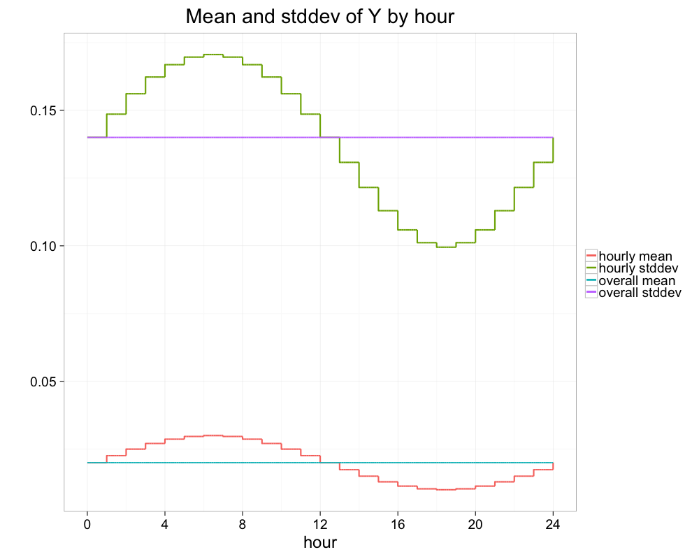 |
| Figure 3: Mean and standard deviation of hourly rate of sessions with purchase |
Variance reduction through prediction
In our previous example, conditioning on hour-of-day slicing did not meaningfully reduce variability. This was a case where our experiment metric was based on a rare binary event, the fraction of user sessions with a purchase. One could argue that we should have included all relevant slicing variables such as country, day of week, customer dimensions (e.g. premium or freemium) etc. Perhaps the combined effect of these factors would be worth addressing? If we were simply to posit the cartesian product of these factors, we would end up with insufficient data in certain cells. A better approach would be to create an explicit prediction of the probability that the user will purchase within a session. We could then define slices corresponding to intervals of the classification probability. To simplify the discussion, assume that all experimental effects are small compared with the prediction probabilities. Of course the classifier cannot use any attributes of the user session that are potentially affected by treatment (e.g. session duration) but that still leaves open a rich set of predictors.
We’d like to get a sense for how the accuracy of this classifier translates into variance reduction. For each user session, say the classifier produces a prediction $\theta$ which is its estimate of the probability of a purchase during that session. $Y$ is the binary event of a purchase. Let’s also assume the prediction is “calibrated” in the sense that $EY|\theta=\theta$, i.e. of the set of user sessions for which the classifier predicts $\theta=0.3$, exactly $30\%$ have a purchase. If $EY=E\theta=\bar{\theta}$ is the overall purchase rate per session, the law of total variance used earlier says that the fraction of variance we cannot reduce by conditioning is
\[
\frac{E_{\theta}[\mathrm{var\ }Y|\theta]}{\bar{\theta}(1-\bar{\theta})}
\]
The mean squared error (MSE) of this (calibrated) classifier is
\[
\frac{E_{\theta}[\mathrm{var\ }Y|\theta]}{\bar{\theta}(1-\bar{\theta})}
\]
The mean squared error (MSE) of this (calibrated) classifier is
\[
E(Y-\theta)^2=E_\theta [\mathrm{var\ }Y|\theta] + E_\theta(EY|\theta - \theta)^2
= E_\theta[\mathrm{var\ }Y|\theta]
\]
In other words, the MSE of the classifier is the residual variance after conditioning. Furthermore, an uninformative calibrated classifier (one which always predicts $\bar{\theta}$) has MSE of $\bar{\theta}(1-\bar{\theta})$. This is equal to $\mathrm{var\ }Y$ so, unsurprisingly, such a classifier gives us no variance reduction (how could it if it gives us a single slice?). Thus, the better the classifier for $Y$ we can build (i.e. the lower its MSE) the greater the variance reduction possible if we condition on its prediction. But since it is generally difficult predict the probability rare events accurately, this is unlikely to be an easy route to variance reduction.
In the previous example, we tried to predict small probabilities. Another way to build a classifier for variance reduction is to address the rare event problem directly — what if we could predict a subset of instances in which the event of interest will definitely not occur? This would make the event more likely in the complementary set and hence mitigate the variance problem. Indeed, I was motivated to take such an approach several years ago when looking for ways to reduce the variability of Google’s search ad engagement metrics. While it is hard to predict in general how a user will react to the ads on any given search query, there are many queries where we can be sure how the user will react. For instance, if we don’t show any ads on a query then there can be no engagement. Since we did not show ads on a very large fraction of queries, I thought this approach appealing and did the following kind of analysis.
Let’s go back to our example of measuring the fraction of user sessions with purchase. Say we build a classifier to classify user sessions into two groups which we will call “dead” and “undead” to emphasize the importance of the rare purchase event to our business model. Suppose the classifier correctly assigns the label “undead” to $100\%$ of the sessions with purchase while correctly predicting “dead” for a fraction $\alpha$ of sessions without purchase. In other words, it has no false negatives and a false positive rate of $1-\alpha$. The idea is to condition on the two classes output by the classifier (again assume we are studying small experimental effects). Let $\theta$ be the fraction of sessions resulting in purchase. The question is how high must $\alpha$ be (as a function of $\theta$) in order to make a significant dent in the variance.
If $w$ is the fraction of sessions for which the classifier outputs “undead”, $w=\theta + (1-\alpha)(1- \theta)$. Meanwhile the conditional variance for the classes “dead” and “undead” are respectively $0$ and $\theta/w \cdot (1-\theta/w)$, leading to an average conditional variance of $w\cdot \theta/w \cdot (1-\theta/w)$. This is the variance remaining of the unconditioned variance $\theta (1-\theta)$. The fractional variance remaining is given by
\[\frac{w \cdot \theta/w \cdot (1 - \theta/w)}{ \theta \cdot (1-\theta)} = \frac{1-\alpha}{1-\alpha+\alpha \theta}
\]
If the probability of a user session resulting in purchase is 2%, a classifier predicting 95% of non-purchase sessions (and all purchase sessions) would reduce variance by 28% (and hence CI widths by 15%). To get a 50% reduction in variance (29% smaller CIs) requires $\alpha \approx 1-\theta$, in this case 98%. Such accuracy seems difficult to achieve if the event of interest is rare.
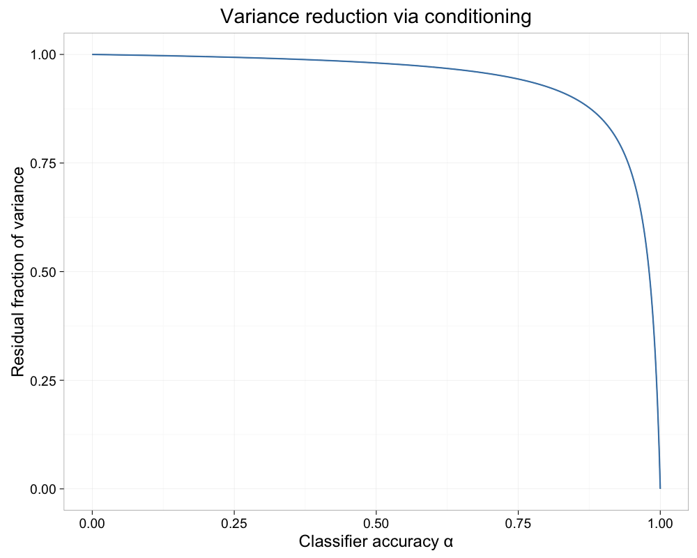 |
| Figure 4: Residual fraction of variance as a function of $\alpha$ when $\theta=2\%$. |
Overlapping (a.k.a factorial) experiments
For one last instance of variance reduction in live experiments, consider the case of overlapping experiments as described in [1]. The idea is that experiments are conducted in “layers” such that a treatment arm and its control will inhabit a single layer. Assignments to treatment and control across layers are independent, leading to what's known as a full factorial experiment. Take the simplest case of two experiments, one in each layer. Every experimental unit (every user session in our example) goes through either Treatment 1 or Control 1 and either Treatment 2 or Control 2. Assuming that the experimental effects are strictly additive, we can get a simple unbiased estimate of the effect of each experiment by ignoring what happens in the other experiment. This relies on the fact that units subject to Treatment 1 and Control 1 on average receive the same treatment in Layer 2.
The effects of Layer 2 on the experiment in Layer 1 (and vice versa) do indeed cancel on average but not in any specific instance. Thus multiple experiment layers introduce additional sources of variability. A more sophisticated analysis could try to take into account the four possible combinations of treatment each user session actually received. Let $Y_i$ be the response measured on the $i$th user session. A standard statistical way to solve for the effects in a full factorial experiment design is via regression. The data set would have a row for each observation $Y_i$ and a binary predictor indicating whether the observation went through the treatment arm of each experiment. When solved with an intercept term, regression coefficients for the binary predictors are maximum likelihood estimates for the experiment effects under assumption of additivity. We could do this but in our big data world, we would avoid materializing such an inefficient structure by reducing the regression to its sufficient statistics. Let
\begin{align}
S_{00} &= \sum_{i \in C_1 \cap C_2} Y_i \\
S_{01} &= \sum_{i \in T_1 \cap C_2} Y_i \\
S_{10} &= \sum_{i \in C_1 \cap T_2} Y_i \\
S_{11} &= \sum_{i \in T_1 \cap T_2} Y_i
\end{align}
Similarly, let $N_{00}=| C_1 \cap C_2 |$ etc. The “regression” estimator for the effect of each experiment are the solutions for $\beta_1$ and $\beta_2$ in the matrix equation
\[\begin{bmatrix}
S_{00}\\
S_{01}\\
S_{10}\\
S_{11}
\end{bmatrix}
=\begin{bmatrix}
N_{00} & 0 & 0 \\
N_{01} & N_{01} & 0\\
N_{10} & 0 & N_{10}\\
N_{11} & N_{11} & N_{11}
\end{bmatrix}
\begin{bmatrix}
\beta_0\\
\beta_1\\
\beta_2
\end{bmatrix}
\]
In contrast, the simple estimator which ignores the other layers has estimates for Experiment 1
\[
\frac{S_{01} + S_{11}}{N_{01}+N_{11}} - \frac{S_{00} + S_{10}}{N_{00}+N_{10}}
\]
and Experiment 2
\frac{S_{01} + S_{11}}{N_{01}+N_{11}} - \frac{S_{00} + S_{10}}{N_{00}+N_{10}}
\]
and Experiment 2
\[
\frac{S_{10} + S_{11}}{N_{10}+N_{11}} - \frac{S_{00} + S_{01}}{N_{00}+N_{01}}
\]
\frac{S_{10} + S_{11}}{N_{10}+N_{11}} - \frac{S_{00} + S_{01}}{N_{00}+N_{01}}
\]
In this example, the regression estimator isn’t very hard to compute, but with several layers and tens of different arms in each layer, the combinatorics grow rapidly. All still doable but we’d like to know if this additional complexity is warranted.
At first blush this problem doesn’t resemble the variance reduction problems in the preceding sections. But if we assume for a moment that Experiment 2’s effect is known, we see that in estimating the effect of Experiment 1, Layer 2 is merely adding variance by having different means in each of its arms. Of course, the effect of Experiment 2 is not known and hence we need to solve simultaneous equations. But even if the effects of Experiment 2 were known, the additional variance due to Layer 2 would be very small unless Experiment 2 has a large effect. And by supposition, we are operating in the LSOS world of very small effects, certainly much smaller than the predictable effects within various slices (such as the 3x effect of hour of day we modeled earlier). Another way to say this is that knowing the effect of Experiment 2 doesn’t help us much in improving our estimate for Experiment 1 and vice versa. Thus we can analyze each experiment in isolation without much loss.
Conclusion
In this post, we continued our discussion from the previous post about experiment analysis in large scale online systems (LSOS). It is often the case that LSOS have metrics of interest based on observations with high coefficients of variation (CV). On the one hand, this means very small effect sizes may be of practical significance. On the other hand, this same high CV makes ineffective some statistical techniques to remove variability due to known or predictable effects.
A different way to frame this is that conditioning reduces measurement variability by removing the effects of imbalance in assigning experimental units within individual slices to treatment and control. This happens because sampling noise causes empirical fractions within slices to deviate from their expectation. At the same time, if the experiment metric is based on observations of high CV, we need to run experiments with a very large number of experimental units in order to obtain statistically significant results. The experiment size is therefore large enough to ensure that the empirical fractions within slices are unlikely to be far from their expectation. In other words, the law of large numbers leaves little imbalance to be corrected by conditioning. All this is just a consequence of conducting sufficiently powerful experiments in a data-rich, information-poor setting.
We conclude this post with two important caveats. First, not all LSOS metrics rely on observations with high CV. For instance, an online music streaming site may be interested in tracking the average listening time per session as an important metric of user engagement. There is no reason a priori to think that listening time per session will have high CV. If the CV is small, the very techniques discussed in this post may improve experiment analysis significantly. Second, this post has explored only a certain class of approaches to reduce measurement variability. Even in the high CV regime, there are techniques which can prove effective though they may require changes to the experiment itself. In a future post we hope to cover the powerful idea of what at Google we call “experiment counterfactuals”.
Until then, if we are operating in a regime where clever experiment analysis doesn’t help, we are freed from having to worry about it. A burden has been lifted. In a way, I find that comforting!
References
[1] Diane Tang, Ashish Agarwal, Deirdre O’Brien, Mike Meyer, “Overlapping Experiment Infrastructure: More, Better, Faster Experimentation”, Proceedings 16th Conference on Knowledge Discovery and Data Mining, Washington, DC
Comments
Post a Comment